Deform 3d методичка

Общее руководство по работе с инженерным программным комплексом DEFORM, Таупек И.М., Кабулова Е.Г., Положенцев К.А., Лисовский А.В., Макаров А.В., 2015

Учебное пособие описывает основные принципы работы с инженерным программным комплексом DEFORM, разработанным американской компанией Scientific Forming Technologies Corporation (SFTC) и предназначенным для анализа технологических процессов обработки металлов давлением и термической обработки. В пособии рассматриваются вопросы подготовки исходных данных для расчёта, включающие особенности подготовки моделей, задания свойств материалов и управления движением рабочим инструментом, а также возможности редактирования встроенной базы данных материалов. Приводятся рекомендации по выполнению моделирования различных процессов ОМД и термообработки. Пособие полезно для инженеров-технологов, научных работников, аспирантов и студентов, занимающихся вопросами и проблемами процессов обработки металлов давлением и термической обработки.

Введение.

DEFORM специализированный инженерный программный комплекс, предназначенный для анализа процессов обработки металлов давлением, термической и механической обработки, разработанный американской компанией Scientific Forming Technologies Corporation (SFTC), являющейся лидером в области моделирования процессов обработки металлов давлением. DEFORM позволяет моделировать практически все процессы, применяемые в обработке металлов давлением (ковка, штамповка, прокатка, прессование и др.), а также операции термической обработки (закалка, старение, отпуск и др.) и механообработки (фрезерование, сверление и др.). Это делает DEFORM мощным инструментом, позволяющим проверить, отработать и оптимизировать технологические процессы, используя на различных этапах исследований только компьютер, а не дорогостоящие эксперименты на производстве. Благодаря этому появляется возможность проверить множество вариантов рассматриваемого процесса, что существенно повышает точность и достоверность полученных результатов исследований, а также возникает возможность буквально заглянуть внутрь заготовки. Программный комплекс применяется по всему миру, как на промышленных предприятиях, так и в научно-исследовательских институтах и технических университетах, является самым распространенным программным комплексом для моделирования процессов обработки металлов давлением, заслуженно считается одной из наиболее точных системой для моделирования сложных трехмерных процессов пластического деформирования металлов.

Содержание.

Введение.
1. Подготовка исходных моделей.
2. Препроцессор DEFORM-3D.
2.1 Загрузка моделей и присвоение свойств материала объектам.
2.2 Настройка конечно-элементной сетки.
2.3 Настройка окон плотности конечно-элементной сетки.
2.4 Настройка граничных условий.
2.5 Настройка параметров расчета.
2.6 Настройка движения объектов.
2.7 Создание базы данных и запуск расчета.
3. Постпроцессор DEFORM-3D.
3.1 Настройка отображения рассчитанных параметров процесса.
3.2 Построение графиков энергосиловых параметров.
3.3 Отображение контактных поверхностей.
3.4 Задание и отслеживание отдельных точек в конечно-элементной сетке.
3.5 Задание координатных сеток.
3.6 Задание разрезов и сечений.
3.7 Настройка многооконного режима.
3.8 Настройка размеров изображения для сохранения результатов.
3.9 Управление и сохранение анимации.
3.10 Настройка различных цветовых схем для шкалы отображения.
4. Использование плоскостей симметрии при моделировании.
5. Использование плоской задачи при моделировании.
5.1 Создание и подготовка применяемых моделей.
5.2 Работа с Препроцессором модуля DEFORM Integrated 2D/3D.
5.3 Работа с Постпроцессором DEFORM Integrated 2D/3D.
6. Создание и редактирование реологических моделей материалов.
7. Моделирование операций термообработки.
7.1 Подготовка моделей.
7.2 Препроцессор модуля «Термическая обработка».
7.3 Просмотр результатов в Постпроцессоре.
8. Особенности моделирования некоторых процессов ОМД.
8.1 Моделирование прокатки.
8.2 Моделирование волочения сплошного профиля.
Библиографический список.
Приложение.

Бесплатно скачать электронную книгу в удобном формате, смотреть и читать:

Скачать книгу Общее руководство по работе с инженерным программным комплексом DEFORM, Таупек И.М., Кабулова Е.Г., Положенцев К.А., Лисовский А.В., Макаров А.В., 2015 — fileskachat.com, быстрое и бесплатное скачивание.

Скачать pdf
Ниже можно купить эту книгу по лучшей цене со скидкой с доставкой по всей России.Купить эту книгу

Скачать
— pdf — Яндекс.Диск.

Дата публикации: 21.02.2022 11:20 UTC

Теги:

Таупек :: Кабулова :: Положенцев :: Лисовский :: Макаров :: 2015 :: DEFORM :: инженерия

Автор:В.С. Паршин, А.П. Карамышев, И.И. Некрасов, А.И. Пугин, А.А. Федулов
Название: Практическое руководство к программному комплексу Deform
Издательство: УРФУ
ISBN: 978-5-321-01772-2
Год: 2010
Формат: JPG
Размер: 391МВ
Страниц:267
Язык:Русский

Учебное пособие посвящено системному описанию принципов работы с программным комплексом DEFORM-3D американской фирмы Scientific Forming Technologies Corporation (SFTC), направленным на проведение конечно-элементного анализа различных технологических процессов металлообработки. Пособие затрагивает вопросы создания инструмента и заготовки, их разбиения конечными элементами, назначения механических свойств, граничных условий, управления работой процессора. Приведены также примеры решения задач с применением рассматриваемого программного комплекса, что придает учебному пособию особую практическую ценность. Пособие полезно для инженеров-разработчиков, научных работников, аспирантов и студентов, в особенности занимающихся исследованиями технологических процессов и оборудования в области обработки металлов давлением.

Автор:

KorovnikovAV · Опубликовано: 23 минуты назад

А потом позвонил
Крокодил
И со слезами просил:
— Мой милый, хороший,
Пришли мне калоши,
И мне, и жене, и Тотоше.

— Постой, не тебе ли
На прошлой неделе
Я выслал две пары
Отличных калош?
— Ах, те, что ты выслал
На прошлой неделе,
Мы давно уже съели
И ждем, не дождемся,
Когда же ты снова пришлешь
К нашему ужину
Дюжину
Новых и сладких калош!

 

Имею спросить, обувью питаешься? 

Чтобы что? На английском говорит 1,5 миллиарда человек, и 90% из них за орфографию и произношенипроизношение учительница города Асбест Свердловской области поставила бы в лучшем случае трояк. Однако все всех понимают. 

Классики говорили «не делайте из еды культа», так вот, перефразирую — » Не делайте из орфографии культа». Если ты душнила по орфографии с тобой никто особо говорить не захочет дальше «пакет нужен»? 

D

EFORM^TM—3D
Лабораторные
работы

1.
Препроцессор

1.1.
Создание новой задачи

1.2.
Установка параметров расчета

1.3.
Загрузка данных объекта

1.4.
Управление экраном

1.5.
Выбор точки

1.6.
Другие кнопки окна Экран (DISPLAY)

1.7.
Сохранение задачи

1.8.
Выход из DEFORM-3D

1.1. Создание новой задачи

На unix-машине введите
DEFORM3 для запуска DEFORM™-3D. На
Windows-машине нажмите кнопку

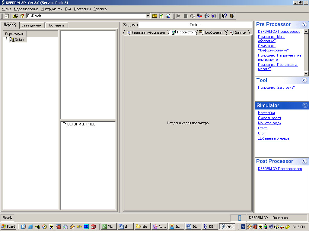
и выберите DEFORM-3D из меню. Откроется
главное (MAIN) окно DEFORM-3D, как показано
ниже.

Создайте новую задачу
выбрав Файл>Новая задача или нажав
кнопку Новая задача

.

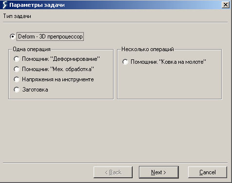
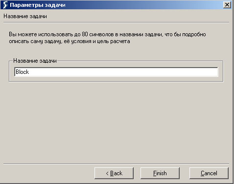
Появиться окно
Параметры задачи. Используйте
установки по умолчанию для запуска
препроцессора DEFORM-3D (не используйте ни
один из мастеров) и нажмите кнопку

.

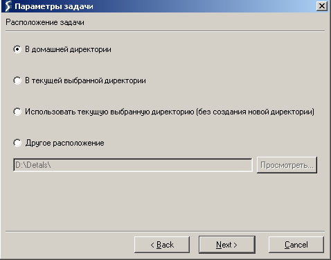
Нажмите кнопку

для определения расположения новой
задачи как ’В домашней директории’.

В поле Название
задачи, введите Block и нажмите
кнопку

.

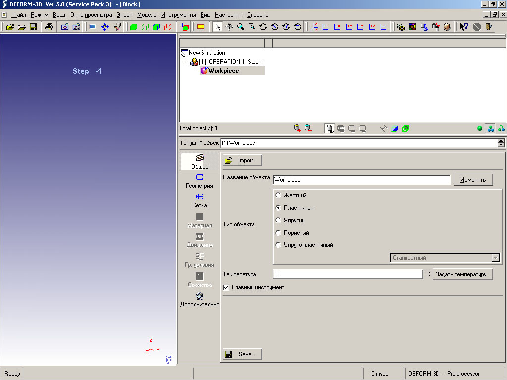
Будет открыт препроцессор
DEFORM-3D. Препроцессор разделен на несколько
различных секций — называемых Экран,
Дерево Объектов и Данные Объектов.
Вверху экрана также находится ряд
кнопок. Эти кнопки будут описаны, так
как они встречаются в лабораторных
работах. Наиболее важные из этих кнопок
находятся справа вверху. Из-за их
важности дается краткое описание
каждой:

Кнопка	Назначение	Описание
	Настройки задачи	В этом меню определяются все параметры расчета и критерии остановки.
	Материал	В этом меню определяются свойства материалов.
	Позиционирование объектов	С помощью этого элемента управления осуществляется позиционирование объектов.
	Взаимодействие объектов	В этом меню определяются отношения между объектами.
	Генерация базы данных	Когда все операции препроцессора выполнены, это меню используется для создания базы данных для расчета.
	Выход	С помощью этой кнопки осуществляется выход из препроцессора и возврат в Главное (MAIN) окно.

Дерево Объектов

Данные Объектов

1 Экран .2. Установка параметров расчета

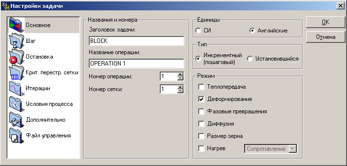
Нажмите кнопку

для открытия окна Настройки задачи.
Измените Заголовок задачи на Block.
Убедитесь, что Единицы измерения
установлены как English и выбран пункт
Деформации (помечен флажком). Для
завершения нажмите кнопку

1.3. Загрузка данных объекта

Добавьте объект в
задачу, нажав кнопку Добавить объект

внизу Дерева объектов. Измените
Название объекта с Object 1 на Block
и нажмите

.
Установите Тип Объекта – Пластичный
(Plastic). В DEFORM поверхность объекта
называется геометрия. Для импорта
геометрии объекта нажмите кнопку

и затем кнопку

.

Самый общий тип файлов
для импорта геометрии в DEFORM-3D –
стереолитография -.STL файл. Геометрия
для блока находится в файле Block_Billet.STL
папке DEFORM3DV5.0Labs. Найдите этот файл,
выберите его и нажмите кнопку

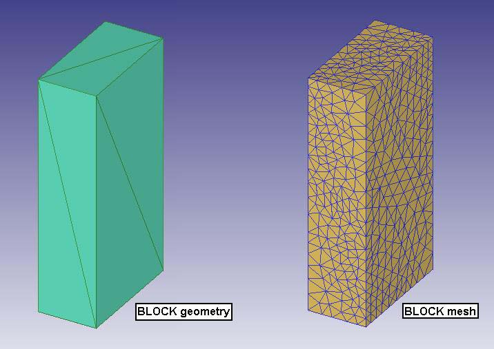
для импорта геометрии в DEFORM. Геометрия
прямоугольного блока должна появиться
Окне экран.

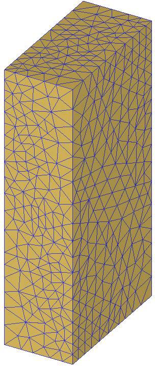
Теперь, когда определена
геометрия Блока, может быть сгенерирована
конечно-элементная сетка объекта.
Нажмите

для открытия окна Управление разбиением
сетки.

Нажмите кнопку

,
чтобы увидеть как выглядит поверхностная
сетка при использовании настроек по
умолчанию. Так как поверхностная сетка
выглядит хорошо, нажмите кнопку

для завершения процесса построения
сетки. Когда построение сетки завершится,
объект должен иметь 5000 элементов,
которые можно увидеть в Дереве Объектов
или в разделе Сводка окна Управление
разбиением сетки.

Соседние файлы в предмете [НЕСОРТИРОВАННОЕ]

• #
• #
• #
• #
• #
• #
• #
• #
• #
• #
• #

Лабораторные работы. — Москва: Инжиниринговая компания Артех, 2008. — 98 с.

DEFORM-3D – мощная система моделирования технологических процессов, предназначенная для анализа трехмерного (3D) поведения металла при различных процессах обработки давлением. DEFORM-3D предоставляет важную информацию о течении материала в штампе и распределении температур во время процесса деформирования.
DEFORM-3D позволяет моделировать такие процессы как: ковка, горячая, полугорячая и холодная штамповка, прессование, прокатка, вытяжка и многие другие процессы.

Содержание

Препроцессор.
Позиционирование инструментов и препроцессор.
Расчет ковки и постпроцессор.
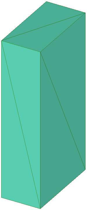
Квадратное кольцо.
Ковка – Перенос от печи к инструменту.
Ковка – Задержка на нижнем штампе.
Ковка – Удар 1.
Ковка – Замена штампа и Удар 2.
Анализ напряженного состояния инструмента.
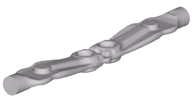
Рулевая тяга.
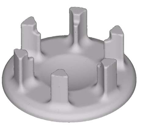
Держатель.
Обжатие (протяжка).

• 1DEFORMTM 3D Version 6.1 (sp1)Users Manual

  Oct 10th 2007

  2545 Farmers Drive, Suite 200Columbus, Ohio, 43235Tel (614)
  451-8330Fax (614) 451-8325Email [email protected]

• 2Table of ContentsPREFACE TO THIS MANUAL
  …………………………………………………………………..6

  Chapter 1. Overview of
  DEFORM…………………………………………………………………….
  71.1 DEFORM family of products
  ……………………………………………………………………………….
  71.2 Capabilities
  ……………………………………………………………………………………………………..
  81.3. Analyzing manufacturing processes with DEFORM
  …………………………………………….. 111.4. Before
  you begin
  ……………………………………………………………………………………………
  111.5. Geometry representation
  …………………………………………………………………………………
  121.6. The DEFORM system
  …………………………………………………………………………………….
  131.7. Pre-processing
  ………………………………………………………………………………………………
  141.8. Creating input data
  …………………………………………………………………………………………
  141.9. File
  system……………………………………………………………………………………………………
  161.10. Running the simulation
  ………………………………………………………………………………….
  171.11. Post-processor
  …………………………………………………………………………………………….
  171.12.
  Units…………………………………………………………………………………………………………..
  18

  Chapter 2. Pre-Processor
  ……………………………………………………………………………..
  192.1. Simulation Controls
  ………………………………………………………………………………………..
  19

  2.1.1. Main controls
  ………………………………………………………………………………………………………
  202.1.2. Step Controls
  ………………………………………………………………………………………………………
  232.1.3. Advanced Step Controls
  ………………………………………………………………………………………..
  262.1.4. Stopping
  Controls…………………………………………………………………………………………………
  292.1.5. Remesh Criteria
  …………………………………………………………………………………………………..
  312.1.6. Iteration
  Controls………………………………………………………………………………………………….
  312.1.7. Processing
  Conditions…………………………………………………………………………………………..
  372.1.8. Advanced Controls
  ……………………………………………………………………………………………….
  392.1.9. Control
  Files………………………………………………………………………………………………………..
  43

  2.2 Material
  Data………………………………………………………………………………………………….
  462.2.1. Phases and
  mixtures…………………………………………………………………………………………….
  472.2.2. Elastic data
  …………………………………………………………………………………………………………
  482.2.3. Thermal
  data……………………………………………………………………………………………………….
  512.2.4. Plastic
  Data…………………………………………………………………………………………………………
  522.2.5. Diffusion
  data………………………………………………………………………………………………………
  612.2.6. Hardness data [MIC]
  …………………………………………………………………………………………….
  632.2.7. Grain growth/recrystallization
  model…………………………………………………………………………
  642.2.8. Advanced material properties
  …………………………………………………………………………………
  702.2.9. Material data requirements
  …………………………………………………………………………………….
  71

  2.3. Inter Material
  Data………………………………………………………………………………………….
  732.3.1. Transformation relation (PHASTF)
  …………………………………………………………………………..
  732.3.2. Kinetics model
  (TTTD)…………………………………………………………………………………………..
  742.3.3. Latent heat
  (PHASLH)…………………………………………………………………………………………..
  792.3.4. Transformation induced volume change (PHASVL)
  …………………………………………………….
  792.3.5. Transformation plasticity
  (TRNSFP)…………………………………………………………………………
  812.3.6. Other Transformation Data
  …………………………………………………………………………………….
  81

• 32.4 Object
  Definition……………………………………………………………………………………………..
  822.4.1. Adding, deleting
  objects…………………………………………………………………………………………
  832.4.2. Object name (OBJNAM)
  ………………………………………………………………………………………..
  842.4.3. Primary Die
  (PDIE)……………………………………………………………………………………………….
  852.4.4. Object type (OBJTYP)
  …………………………………………………………………………………………..
  852.4.5. Object
  geometry…………………………………………………………………………………………………..
  872.4.6. Object meshing
  ……………………………………………………………………………………………………
  952.4.7. Object material
  …………………………………………………………………………………………………..
  1072.4.8. Object initial
  conditions………………………………………………………………………………………..
  1072.4.9. Object
  properties………………………………………………………………………………………………..
  1082.4.10. Object boundary
  conditions…………………………………………………………………………………
  1152.4.11. Contact boundary
  conditions……………………………………………………………………………….
  1182.4.12. Object movement controls
  ………………………………………………………………………………….
  1182.4.13. Object node
  variables……………………………………………………………………………………….
  1312.4.14. Object element variables
  …………………………………………………………………………………..
  138

  2.4.16. Data Interpolation
  …………………………………………………………………………………
  1452.5.1. Inter object
  Interface…………………………………………………………………………………………..
  1492.5.2. Positioning
  ……………………………………………………………………………………………………….
  1622.5.3. Inter object boundary conditions
  …………………………………………………………………………..
  164

  2.6. Database Generation
  …………………………………………………………………………………..
  165Chapter 3. Running Simulations
  …………………………………………………………………..
  167

  3.1. Simulation Options
  ……………………………………………………………………………………….
  1683.2. Switching between Solvers (Conjugate-Gradient and
  Sparse)……………………………………. 168

  3.3. Multi Processing
  …………………………………………………………………………………………..
  1693.3. Email the Result
  ………………………………………………………………………………………….
  1703.4. Starting the simulation
  ………………………………………………………………………………….
  1703.5. Simulation graphics
  ………………………………………………………………………………………
  1713.6. Add to Queue (Batch Queue)
  …………………………………………………………………………
  1723.7 Process Monitor
  ………………………………………………………………………………………….
  1733.8. Stopping a simulation
  ……………………………………………………………………………………
  1743.9. Troubleshooting problems
  ……………………………………………………………………………..
  174

  3.9.1. Message file messages
  ……………………………………………………………………………………….
  1743.9.2. Simulation aborted by user
  …………………………………………………………………………………..
  1743.9.3. Cannot remesh at a negative
  step………………………………………………………………………….
  1753.9.4. Remeshing is highly
  recommended………………………………………………………………………..
  1753.9.5Negative
  Jacobian………………………………………………………………………………………………..
  1753.9.6. Solution does not converge
  ………………………………………………………………………………….
  1763.9.7. Stiffness matrix is non-positive
  definite……………………………………………………………………
  1793.9.8. Zero
  pivot………………………………………………………………………………………………………….
  1793.9.9. Extrapolation of data
  …………………………………………………………………………………………..
  1793.9.10. Bad Element
  Shape…………………………………………………………………………………………..
  1803.9.11. Inconsistent Step
  Number…………………………………………………………………………………..
  181

  Chapter 4: Post-Processor
  ………………………………………………………………………….
  1824.1.Post-Processor Overview
  ……………………………………………………………………………….
  1834.2 Graphical
  display…………………………………………………………………………………………..
  184

  4.2.1. Window
  layout……………………………………………………………………………………………………
  184

• 44.3.Post-Processing Summary
  ……………………………………………………………………………..
  1934.3.1.Simulation Summary
  ……………………………………………………………………………………………
  1934.3.2.State Variable
  …………………………………………………………………………………………………….
  195Displacement……………………………………………………………………………………………………………..
  200Density……………………………………………………………………………………………………………………..
  200Strain
  ……………………………………………………………………………………………………………………….
  200Velocity
  …………………………………………………………………………………………………………………….
  202Normal
  Pressure…………………………………………………………………………………………………………
  202Temperature………………………………………………………………………………………………………………
  202Volume Fraction
  …………………………………………………………………………………………………………
  202Grain Size
  …………………………………………………………………………………………………………………
  203Hardness…………………………………………………………………………………………………………………..
  203Dominant atom
  …………………………………………………………………………………………………………..
  203User
  Variables……………………………………………………………………………………………………………
  2034.3.3.Point tracking
  ……………………………………………………………………………………………………..
  2034.3.4.Load stroke
  curves………………………………………………………………………………………………
  2054.3.5.Coordinate Systems
  …………………………………………………………………………………………….
  2064.3.6. Step Selection & Manipulation
  ……………………………………………………………………………..
  2074.3.7. Steps list
  ………………………………………………………………………………………………………….
  2084.3.8.View Changes Within Viewport
  ………………………………………………………………………………
  2104.3.9. Coordinate System
  Selection………………………………………………………………………………..
  2104.3.10.Rotation
  …………………………………………………………………………………………………………..
  2114.3.11.Coordinate Axis View
  …………………………………………………………………………………………
  2114.3.12.Point Selection
  ………………………………………………………………………………………………….
  2114.3.13 Multiple Viewports
  ……………………………………………………………………………………………..
  2124.3.14. Nodes
  …………………………………………………………………………………………………………….
  2124.3.15.
  Elements………………………………………………………………………………………………………..
  2134.3.16.
  Viewport…………………………………………………………………………………………………………
  2154.3.17. Data
  Extraction…………………………………………………………………………………………………
  2174.3.18.Flownet……………………………………………………………………………………………………………
  2184.3.19. Mirroring
  ………………………………………………………………………………………………………..
  2224.3.20 Animation controls and saving.
  …………………………………………………………………………….
  223

  Chapter 5: Elementary Concepts in Metalforming and Finite
  Element Analysis …… 225Chapter 6: User Routines
  ……………………………………………………………………………
  237

  User-Defined FEM
  Routines………………………………………………………………………………………….
  237User-Defined Post-Processing Routines
  ………………………………………………………………………….
  241

  6.1. User defined FEM routines
  ……………………………………………………………………………
  2416.2. User defined post-processing routines
  …………………………………………………………….
  267

  Quick
  Reference…………………………………………………………………………………………
  273Hot
  Forming……………………………………………………………………………………………….
  276

  Appendix A: Running DEFORM in text
  mode………………………………………………………….
  283Appendix B: Inserting DEFORM Animations in Powerpoint
  Presentations ……………….. 287Appendix C: DETAILS OF
  MOVEMENT CONTROLS IN SPIN.KEY …………………………..
  289Appendix D: Data
  Files……………………………………………………………………………………….
  291Appendix E: 2D to 3D Conversion
  Utility………………………………………………………………..
  293Appendix F: Fracture with Element Deletion and Damage
  Softening………………………….. 295

• 5Appendix G: Rotating Work piece Simulations
  ………………………………………………………..
  300Appendix H: Sheet Forming in DEFORM-3D
  ………………………………………………………….
  308Appendix I: Eulerian treatment of the 3D rolling process
  ………………………………………….. 317Appendix J:
  Preventing leakage of nodes in sectioned simulations
  ……………………………. 318Appendix K: The Double
  Concave Corner Constraint
  ……………………………………………… 321Appendix
  L: Rolling Simulation Overview (In
  Progress)…………………………………………….
  324Appendix M: Checking the forming loads results of a simulation
  ……………………………….. 326Appendix N: Model setup
  for steady state machining
  ……………………………………………… 328Appendix
  O: Document on constructing linear friction
  simulations……………………………… 336Appendix P: On
  Using Spring-Loaded Dies
  ……………………………………………………………
  345Appendix Q: THE DEFORM ELASTO-PLASTIC
  MODEL…………………………………………. 347Appendix
  R: Setting Up Multiple Processor
  Simulations……………………………………………
  353Appendix S: Coupled Die Stress Analysis…356Appendix T: Setting
  up steady state extrusion357Appendix U: Setting up 3D machining
  models365

• 6Preface to this manualThis manual describes the features and
  capabilities of the DEFORM-3D system.It also contains a description
  of the inputs and actions required to setup problemsand run
  simulations. If you have not used DEFORM before we would
  recommendthat you go through the lab manuals first for an
  introduction on how to use thesystem and how to run different types
  of simulations. The labs for DEFORM-3D,DEFORM-HT are provided as
  PDF (Portable document format) documents whichcan be viewed using
  Adobe Acrobat provided with DEFORM. All keywords whichare used in
  DEFORM-3D are documented in the keyword reference manualswhich are
  also provided as a PDF document. All documents can be accessedfrom
  the help menus in the main program, pre-processor, and
  post-processor.

  Overview of DEFORMPresents an overview of the DEFORM family of
  products.

  Analyzing manufacturing processes with DEFORMDescribes how to
  use DEFORM products to analyze manufacturingprocesses.

  The DEFORM systemIntroduces the DEFORM-3D system and describes
  the components thatmake up the system.

  Pre-ProcessorDescribes the layout of the DEFORM
  Pre-Processor.

  Running SimulationsDescribes how to run simulations and also how
  to handle errors that occurduring simulations.

  Post-ProcessorDescribes post-processing results from simulations
  and how to interpretresults.

  User RoutinesDescribes user FORTRAN routines in detail. DEFORM
  allows the user towrite FORTRAN programs to describe the flow
  stress, die speeds, damageaccumulation, and other features, as well
  as defining and storing newvariables which can be tracked in the
  post-processor along with the standardDEFORM variables.

  Release NotesContains release notes.

• 7Chapter 1. Overview of DEFORMDEFORM is a Finite Element Method
  (FEM) based process simulation systemdesigned to analyze various
  forming and heat treatment processes used bymetal forming and
  related industries. By simulating manufacturing processes ona
  computer, this advanced tool allows designers and engineers to:

  Reduce the need for costly shop floor trials and redesign of
  tooling andprocesses.

  Improve tool and die design to reduce production and material
  costs.

  Shorten lead time in bringing a new product to market.Unlike
  general purpose FEM codes, DEFORM is tailored for
  deformationmodeling. A user friendly graphical user interface
  provides easy data preparationand analysis so engineers can focus
  on forming, not on learning a cumbersomecomputer system. A key
  component of this is a fully automatic, optimizedremeshing system
  tailored for large deformation problems.DEFORM-HT adds the
  capability of modeling heat treatment processes,including
  normalizing, annealing, quenching, tempering, aging, and
  carburizing.DEFORM-HT can predict hardness, residual stresses,
  quench deformation, andother mechanical and material
  characteristics important to those that heat treat.

  1.1 DEFORM family of products

  DEFORM-2D (2D)Available on UNIX/LINUX platforms (HP, DEC, LINUX)
  as well as personalcomputers running Windows-XP/Vista. Capable of
  modeling plane strain oraxisymmetric parts with a simple 2
  dimensional model. A full function packagecontaining the latest
  innovations in Finite Element Modeling, equally well suitedfor
  production or research environments.

  DEFORM-3D (3D)Available on UNIX/LINUX platforms (HP, DEC, LINUX)
  as well as personalcomputers running Windows-XP/Vista.DEFORM-3D is
  capable of modelingcomplex three dimensional material flow
  patterns. Ideal for parts which cannot besimplified to a two
  dimensional model.

  DEFORM-F2 (2D)Available on personal computers running Windows
  XP/Vista. Capable ofmodeling-two dimensional axisymmetric or plane
  strain problems. Suitable forsmall to mid-sized shops starting in
  Finite Element Modeling.

  DEFORM-F3 (3D)Available on personal computers running Windows
  XP/Vista. A powerful three-dimensional modeling package for
  modeling cold, warm and hot forgingprocesses.

• 8DEFORM-HTAvailable as an add-on to DEFORM-2D and DEFORM-3D. In
  addition to thedeformation modeling capabilities, DEFORM-HT can
  model the effects of heattreating, including hardness, volume
  fraction of metallic structure, distortion,residual stress, and
  carbon content.

  1.2 Capabilities

  Deformation

  Coupled modeling of deformation and heat transfer for simulation
  of cold,warm, or hot forging processes (all products).

  Extensive material database for many common alloys including
  steels,aluminums, titaniums, and super-alloys (all products).

  User defined material data input for any material not included
  in thematerial database (all products).

  Information on material flow, die fill, forging load, die
  stress, grain flow,defect formation and ductile fracture (all
  products).

  Rigid, elastic, and thermo-viscoplastic material models, which
  are ideallysuited for large deformation modeling (all
  products).

  Elastic-plastic material model for residual stress and spring
  backproblems. (2D, 3D).

  Porous material model for modeling forming of powder
  metallurgyproducts (2D, 3D).

  Integrated forming equipment models for hydraulic presses,
  hammers,screw presses, and mechanical presses (all products).

  User defined subroutines for material modeling, press modeling,
  fracturecriteria and other functions (2D, 3D).

  FLOWNET (2D, PC,) and point tracking (all products) for
  importantmaterial flow information.

  Contour plots of temperature, strain, stress, damage, and other
  keyvariables simplify post processing (all products).

  Self contact boundary condition with robust remeshing allows a
  simulationto continue to completion even after a lap or fold has
  formed (2D, 3D).

  Multiple deforming body capability allows for analysis of
  multipledeforming work pieces or coupled die stress analysis. (2D,
  3D).

  Fracture initiation and crack propagation models based on well
  knowndamage factors allow modeling of shearing, blanking, piercing,
  andmachining (2D, 3D).

• 9Heat Treatment Simulate normalizing, annealing, quenching,
  tempering, and carburizing.

  Normalizing (not available yet)Heating a ferrous alloy to a
  suitable temperature above the transformationrange and cooling in
  air to a temperature substantially below thetransformation
  range.Annealing A generic term denoting a treatment, consisting of
  heating to and holdingat a suitable temperature followed by cooling
  at a suitable rate, usedprimarily to soften metallic materials. In
  ferrous alloys, annealing usually isdone above the upper critical
  temperature, but the time-temperaturecycles vary both widely in
  both maximum temperature attained and incooling rate
  employed.Tempering (not available yet)Reheating hardened steel or
  hardened cast iron to some temperaturebelow the eutectoid
  temperature for the purpose of decreasing hardnessand increasing
  toughness.Stress relievingHeating to a suitable temperature,
  holding long enough to reduce residualstresses, and then cooling
  slowly enough to minimize the development ofnew residual
  stresses.QuenchingA rapid cooling whose purpose is for the control
  of microstructure andphase products.

  Predict hardness, volume fraction metallic structure,
  distortion, and carboncontent.

  Specialized material models for creep, phase transformation,
  hardnessand diffusion.

  Jominy data can be input to predict hardness distribution of the
  finalproduct.

  Modeling of multiple material phases, each with its own elastic,
  plastic,thermal, and hardness properties. Resultant mixture
  material propertiesdepend upon the percentage of each phase present
  at any step in theheat treatment simulation.

  DEFORM models a complex interaction between deformation,
  temperature, and,in the case of heat treatment, transformation and
  diffusion. There is couplingbetween all phenomenon, as illustrated
  in the figure below. When appropriatemodules are licensed and
  activated, these coupling effects include heating due todeformation
  work, thermal softening, and temperature controlled
  transformation,latent heat of transformation, transformation
  plasticity, transformation strains,stress effects on
  transformation, and carbon content effects on all
  materialproperties.

• 10

  Figure 1.2.1 : Relationship between various DEFORM modules.

• 11

  1.3. Analyzing manufacturing processes with DEFORMDEFORM can be
  used to analyze most thermo-mechanical forming processes,and many
  heat treatment processes. The general approach is to define
  thegeometry and material of the initial work piece in DEFORM, then
  sequentiallysimulate each process that is to be applied to the work
  piece.The recommended sequence for designing a manufacturing
  process usingDEFORM

  Define your proposed process Final forged part geometry Material
  Tool progressions Starting work piece/billet geometry Processing
  temperatures, reheats, etc. Gather required data Material data
  Processing condition data Using the DEFORM pre-processor, input the
  problem definition for the

  first operation Submit the data for simulation Using the DEFORM
  post-processor, review the results Repeat the
  preprocess-simulate-review sequence for each operation in

  the process If the results are unacceptable, use your
  engineering experience and

  judgment to modify the process and repeat the simulation
  sequence.1.4. Before you beginBefore you begin work on your DEFORM
  simulation, spend some time planningthe simulation. Consider the
  type of information you hope to gain from theanalysis. Are
  temperatures important? What about die fill? Press loads?
  Materialdeformation patterns? Ductile fracture of the part? Die
  failure? Buckling? Can thepart be modeled as a two dimensional
  part, or is a three dimensional simulationnecessary? Having a
  definite goal will help you design a simulation which willprovide
  the information most vital to understanding your manufacturing
  process.

• 12

  1.5. Geometry representation

  Figure 1.5.1 : Axisymmetric and plane strain examples.

  DEFORM simulations can be run either as two dimensional (2D) or
  threedimensional (3D) models. In general, 2D models are smaller,
  easier to set up,and run more quickly than 3D models. Frequently,
  the added detail of a 3Dmodel is not worth the additional time
  required over a 2D simulation if theprocess can reasonably be
  represented in 2D.There are two 2D geometry representations:
  axisymmetric and plane strain.Axisymmetric geometries assume that
  the geometry of every plane radiating outfrom the centerline is
  identical. Plane strain requires that there is no material flowin
  the out of plane direction, and that flow in every plane parallel
  to the sectionmodeled is identical. Figure 1.5.1 illustrates
  axisymmetric and plane strainmodels.Objects that are closely
  approximated by axisymmetric or plane strain modelscan also be
  modeled in 2D by neglecting minor variations. For example, if
  thehead shape is not critical a hex head bolt can be modeled as
  axisymmetric bydefining a head radius which maintains constant
  volume (radius =0.525*(distance across flats)). A gradually
  tapering part such as a turbine bladecan be modeled by modeling
  several plane strain sections.

• 13

  Figure 1.5.2 : Buckling.

  Buckling of cylindrical parts is a fully three dimensional
  process, and must bemodeled as such if such behavior is expected.
  An axisymmetric simulation willnot show buckling; even if it will
  occur in the actual process (Figure 1.5.2 ).Partswhich cannot be
  simplified to 2D must be modeled as 3D.

  1.6. The DEFORM systemThe DEFORM system consists of three major
  components:

  1. A pre-processor for creating, assembling, or modifying the
  data required toanalyze the simulation, and for generating the
  required database file.

  2. A simulation engine for performing the numerical calculations
  required toanalyze the process, and writing the results to the
  database file. Thesimulation engine reads the database file,
  performs the actual solutioncalculation, and appends the
  appropriate solution data to the databasefile. The simulation
  engine also works seamlessly with the AutomaticMesh Generation
  (AMG) system to generate a new FEM mesh on thework piece whenever
  necessary. While the simulation engine is running, itwrites status
  information, including any error messages, to the message(.MSG) and
  log (.LOG) files.

  3. A post-processor for reading the database file from the
  simulation engineand displaying the results graphically and for
  extracting numerical data.

• 14

  1.7. Pre-processingThe DEFORM preprocessor uses a graphical user
  interface to assemble the datarequired to run the simulation. Input
  data includes

  Object descriptionIncludes all data associated with an object,
  including geometry, mesh,temperature, material, etc.

  Material dataIncludes data describing the behavior of the
  material under the conditionswhich it will reasonably experience
  during deformation.

  Inter object conditionsDescribes how the objects interact with
  each other, including contact, friction,and heat transfer between
  objects.

  Simulation controlsIncludes instructions on the methods DEFORM
  should use to solve theproblem, including the conditions of the
  processing environment, whatphysical processes should be modeled,
  how many discrete time steps shouldbe used to model the process,
  etc.

  Inter material dataDescribes the physical process of one phase
  of a material transforming intoother phases of the same material in
  a heat treatment process. For example,the transformation of
  austenite into pearlite, banite, and martensite.

  1.8. Creating input dataThere are several ways to enter data
  into the DEFORM pre-processor.Depending on the requirements of a
  particular problem, a combination of thefollowing methods will
  frequently be used.

  Manual inputThe pre-processor menus contain input fields for
  nearly every possible data inputin DEFORM. The user can enter,
  view, or edit any of these values. Discussionsof each field are
  contained in the reference section of this manual.

  Keyword file inputMost of the data fields in the DEFORM
  pre-processor correspond directly to aDEFORM keyword. Individual
  keywords describe very specific information abouta particular
  object characteristic, simulation control, material characteristic,
  orinter-object relationship. Keyword data can be saved in a keyword
  (.KEY) file. A

• 15

  keyword file is a human readable (ASCII) representation of
  DEFORM simulationdata.The typical format of a keyword is:[keyword
  name] [keyword parameters][default data][data][data]…A keyword
  file may contain a complete simulation data set, or it may contain
  onlyone or a few specific keywords.

  Assembling keyword filesWhen a keyword file is read into the
  pre-processor, only the specific data fieldslisted in that keyword
  are changed; the remainder is unchanged. Thus, it ispossible to
  assemble a complete set of problem data by loading one keyword
  filethat contains only data for one object, another keyword file
  that contains materialdata, etc.To save specific elements of a
  keyword file, it is necessary to save the entire file,then use a
  text editor such as Notepad, VI, emacs, or equivalent to
  deleteunwanted information. The keyword file load and save features
  on the main pre-processor menu load or save an entire data set. To
  load partial keyword files,use the Keyword, Load option from the
  File menu.

  Other file inputsVarious data types, particularly part
  geometries and material data, can be readfrom appropriate format
  files.

  Modifying problem dataSolution or input step data from any
  stored step in a database file can be readinto the pre-processor,
  modified, and either appended to an existing database, orwritten to
  a new database file.

  Viewing specific problem dataMost problem data stored in the
  database file is accessible in the post-processor.However, certain
  specific information such as boundary conditions or
  inter-objectcontact conditions is displayed differently in the
  pre-processor. When debugginga problem which is not running
  properly, it is sometimes useful to use the pre-processor data
  display to view this information.

• 16

  1.9. File systemThe primary data storage structure is the
  database file. The database file storesa complete set of simulation
  data, including object data, simulation controls,material data, and
  inter-object relations, both from the original input, and
  fromselected solution steps. The sequence of information storage in
  a database file isshown in Figure 1.9.1 . The pre-processor uses an
  ASCII format file called thekeyword file to create inputs.

  Figure 1.9.1 : DEFORM database structure.

  Each DEFORM problem has an associated problem ID and should be
  created inits own folder or directory. For every problem, the
  DEFORM system creates fourtypes of files that are generally
  accessible to users:

  Database (DB) filesThe database file contains the complete
  simulation data set for input data andeach saved simulation step.
  The information is stored in a compressed, machinereadable format,
  and is accessible only through the DEFORM pre- and post-processors.
  As the simulation runs, data for each step is written to the end of
  thedatabase file. If the step being written is specified as a step
  to be saved,information for the next step will be appended after
  the current data step. If thestep is not specified to be saved, and
  a solution is found for the next step, thedata for the current step
  will be overwritten by the data for the next step.

• 17

  Keyword (KEY) filesKeyword files contain specific problem
  definition data which is read by the pre-processor and used to
  create an input database file. A keyword file may containa complete
  problem definition, or it may contain only specific information
  about,for example, a specific object or material. The information
  is stored in ASCIIformat, and can be read and edited with any text
  editor, such as Notepad, VI, oremacs. A keyword reference is
  available which describes the data format foreach keyword.

  1.10. Running the simulation

  Simulation engineThe simulation engine is the program which
  actually performs the numericalcalculations to solve the problem.
  The simulation engine reads input data fromthe database, then
  writes the solution data back out to the database. As it runs,
  itcreates two user readable files which track its progress.

  Log (LOG) filesLog files are created when a simulation is
  running. They contain generalinformation on starting and ending
  times, remeshings (if any), and may containerror messages if the
  simulation stops unexpectedly.

  Message (MSG) filesMessage files are also created when a
  simulation is running. They containdetailed information about the
  behavior of the simulation, and may containinformation regarding
  why a simulation has stopped.

  1.11. Post-processor

  The postprocessor is used to view simulation data after the
  simulation has beenrun. The postprocessor features a graphical user
  interface to view geometry, fielddata such as strain, temperature,
  and stress, and other simulation data such asdie loads. The
  postprocessor can also be used to extract graphic or numericaldata
  for use in other applications.

• 18

  1.12. UnitsDEFORM data may be supplied in any unit system, as
  long as all variables areconsistent (i.e., length, force, time, and
  temperature measurements are in thesame units, and all derived
  units — such as velocity — are derived from the samebase units).
  This task can be simplified by using either the British or SI
  system forthe default unit system.

  Figure 1.12.1 : DEFORM unit system.

  Note: It is important to select the unit system at the beginning
  of the simulation.Once numerical values have been entered in the
  pre-processor, the numericalvalues will remain unchanged even if
  the unit system designation is changed.

  The Post-Processor has been equipped with a feature for unit
  conversion fordatabase viewing. The user has four options for unit
  conversion. If the conversionfactor selected is Default, then the
  units are picked up automatically dependingon whether the database
  is English or SI. Since there is no conversionnecessary, all the
  conversion factors are set to 1.0 in this column. For the casesof
  converting English to SI or converting SI to English, the
  conversion factors andunits are picked up from the dialog and the
  values are converted and displayed inthe post-processor. The fourth
  option gives the user the option of viewing thedata from the
  database in units that are not English or SI. The user is free
  toenter the conversion factors and the units corresponding to the
  conversionfactors. There is no user type unit conversion for
  temperature, since thetemperature conversion is not a simple
  multiplication.

• 19

  Chapter 2. Pre-Processor

  Figure 2.1.0 : The preprocessor of DEFORM-3D. The simulation
  controls button ishighlighted with a red square.

  2.1. Simulation ControlsThe Simulation Controls window can be
  found by clicking a button in thePreprocessor ( ). Options defined
  under Simulation Controls (See Figure2.1.1 ) control the numerical
  behavior of the solution. Main controls details withspecifying the
  simulation title, unit system, geometry type, etc. Stopping and
  stepcontrols are used to specify the time step, the total number of
  steps and thecriteria used to terminate the simulation. Processing
  conditions like theenvironment temperature, convection coefficient
  can be specified underProcessing conditions. Certain advanced
  features are explained in the Advancedcontrols section.

• 20

  Figure 2.1.1 : Simulation Controls window.

  2.1.1. Main controls

  Simulation title (TITLE)The simulation title allows you to title
  the problem (up to 80 characters) forreference purposes.

  Operation name (SIMNAM)The operation name allows you to title
  the specific operation (up to 80characters) for reference
  purposes.Units (UNIT)The DEFORM unit system can be defined as
  English or Metric (SI). Allinformation in DEFORM should be
  expressed in consistent units. The unit systemshould be selected at
  the beginning of the problem setup procedure, and shouldnot be
  changed during a simulation or after an operation.

• 21

  Figure 2.1.2 : DEFORM unit system.

  Type

  The five different types of simulations that can be run are:

  Lagrangian Incremental: To be used for all the conventional
  forming, heattransfer and heat-treat applications. Transient phase
  of the processes likerolling, machining, extrusion, drawing cogging
  etc. also can be modeled inthis general framework.

  ALE Rolling: ALE model for rolling process can be generated
  using theShape Rolling template. When the model is generated using
  thistemplate, automatically generates the necessary boundary
  conditions forthe entry surface for the billet (indicated in the
  interface as the Beginningsurface, nodes are assigned BCCDEF=4),
  and the exit surface ( indicatedin the interface as Free surface,
  nodes are assigned BCCDEF=5).Template automatically sets the
  analysis type as ALE Rolling. When therolling model is setup using
  the regular pre-processor, user needs to setthis analysis type and
  proper boundary conditions to be able to run theALE model for
  rolling.

  Steady-State machining: 3D machining model for turning
  applications canbe generated using the Machining Template in which
  the initial model canbe set up for Lagrangian Incremental run. When
  sufficient chip has formedthe template can be used to generate an
  additional operation to switch theanalysis mode to Steady State. In
  this stage template can be used togenerate the required boundary
  conditions for the steady state run, whichincludes defining end
  surface of the chip (indicated as free surface, withBCCDEF code set
  as 5 for those nodes). Template automatically sets theanalysis type
  as Steady-State Machining. When the machining model issetup using
  the regular pre-processor, user needs to set this analysis typeand
  proper free surface and thermal boundary conditions to be able to
  runthe Steady State model for machining.

• 22

  Ring Rolling: From 3DV61, simulation engine has been enhanced
  tohandle the non isothermal modeling of ring rolling process.
  Thisdevelopment includes a special ALE technique that does not
  depend onany expensive computing resources, nor involves very long
  modelingtimes.

  Steady-State extrusion: Provided for future implementation:
  (CurrentEulerian process modeling capability for extrusion, which
  is underdevelopment can be activated using a special data file
  called ALE.DAT.Please contact SFTC for additional information.)

  Simulation modes (SMODE, TRANS)DEFORM features a group of
  simulation modes that may be turned on or offindividually, or used
  in various combinations.

  Heat transferSimulates thermal effects within the simulation,
  including heat transferbetween objects and the environment, and
  heat generation due todeformation or phase transformation, where
  applicable.

  DeformationSimulates deformation due to mechanical, thermal, or
  phase transformationeffects.

  TransformationSimulates transformation between phases due to
  thermomechanical and timeeffects.

  DiffusionSimulates diffusion of carbon atoms within the
  material, due to carboncontent gradients.

  GrainSimulates grain size calculation and recrystallization
  calculations.

  HeatingSimulates heat generation due to resistance or induction
  heating. Thisfeature is not activated in the current release.

• 23

  For backward compatibility with old keywords and databases,
  before version3.0, the keyword SMODE (old style isothermal,
  non-isothermal, heat transfer)is read and the corresponding keyword
  TRANS mode switches are set in thepre-processor.

  Operation number (CURSIM)Allows the specification of a new
  operation number for each simulation in thedatabase. If operations
  numbers are specified, the post-processor displays eachoperation
  with its number in the step list.

  Mesh number (MESHNO)This variable records the current mesh based
  on the number of remeshings thatoccur between the initial mesh and
  the current mesh. This variable should not bechanged.

  Figure 2.1.3 : Step Controls.

  2.1.2. Step ControlsThe DEFORM system solves time dependent
  non-linear problems by generatinga series of FEM solutions at
  discrete time increments. At each time increment,the velocities,
  temperatures, and other key variables of each node in the
  finiteelement mesh are determined based on boundary conditions,
  thermomechanicalproperties of the work piece materials and possibly
  solutions at previous steps.Other state variables are derived from
  these key values, and updated for eachtime increment. The length of
  this time step, and number of steps simulated, aredetermined based
  on the information specified in the step controls menu (See

• 24

  Figure 2.1.3 ).Starting step number (NSTART)

  If a new database is written, the specified step number will be
  the first step in thedatabase. If data is written to an existing
  database, the preprocessor data will beappended to this database in
  proper numerical order, and any steps after the onespecified will
  be overwritten.The negative (-n) flag on the step number indicates
  that the step was written tothe database by the pre-processor
  (either by manual generation of a databasestep or by an automatic
  remesh), not by the simulation engine.Note: All pre-processor
  generated steps should have a negative step number

  Number of simulation steps (NSTEP)

  The number of simulation steps parameter defines the number of
  steps to runfrom the starting step number. The simulation will stop
  after this number ofsimulation steps will have run, if another
  stopping control is triggered to stop thesimulation or if the
  simulation runs into a problem. For example, if the startingstep
  number is -35 (NSTART), and 30 steps (NSTEP) are specified,
  thesimulation will stop after the 65th step, unless another
  stopping control istriggered first.

  Step increment to save (STPINC)

  The step increment to save in the database controls the number
  of steps that thesystem will save in the database. When a
  simulation runs, every step must becomputed, but does not
  necessarily need to be saved in the database. Storingmore steps
  will preserve more information about the process; consequently it
  willrequire more storage space.

  Primary die (PDIE)

  The primary die is the object for which many stopping and
  stepping criteria aredefined. For example, stopping distance based
  on primary die stroke. When thestroke of the object defined as the
  primary die reaches the value for primary diedisplacement, the
  simulation will be stopped whether or not more steps werespecified.
  The Step By Stroke feature determines step size based on
  themovement of the primary die.The primary die is usually assigned
  to the object most closely controlled by theforging machinery. For
  example, the die attached to the ram of a mechanicalpress would be
  designated as the primary object.

• 25

  Step increment control (DSMAX/DTMAX)

  Solution step size can be controlled by time step or by
  displacement of theprimary die. If stroke per step is specified,
  the primary die will move the specifiedamount in each time step.
  The total movement of the primary die will be thedisplacement per
  step multiplied by the total number of steps. If time per step
  isspecified, the time interval per step will be used. The die
  displacement per stepwill be the time step times the die
  velocity.From 3DV61, the definition of step increment control has
  been enhanced toinclude both the time and stroke dependent step
  functions. This means, step size(both time per step and stroke per
  step) can now be defined as a function of timeor stroke. This
  functionality enables finer resolution of saved model
  information,where it is desired. (Typically towards the end of the
  stroke, where steepchanges of die load and cavity filling or flash
  formation can take place).Stroke per step is frequently more
  intuitive. However, time per step must bespecified for any problem
  in which there is no die movement (such as heattransfer), or for
  any problem where force control is used.Selecting time step and
  number of stepsProper time step selection is important. Too large a
  time step can causeinaccuracy in the solution, rapid mesh
  distortion or convergence problems. Toosmall a time step can lead
  to unnecessarily long solution times. The followingsection provides
  some guidelines for selecting time steps.The maximum displacement
  for any node should not exceed about 1/3 the lengthof its element
  edge length in one step. For flow around a tight corner,
  flashforming, or similar highly localized deformations, time steps
  may need to bedefined to give a node movement of as small as 1/10
  or the element edge length.Thus, for a finer mesh, smaller steps
  are required than for a coarser mesh. Thisprevents the mesh from
  becoming overly distorted in a single time step.The time step can
  be determined by the following method:

  1. Using the measurement tool, measure one of the smaller
  elements in thedeforming object (this must be done after a mesh has
  been generated)

  2. Estimate the maximum velocity of any region of the work piece
  (for mostproblems, this will be the die velocity. For extrusion
  problems it will be thedie velocity times the extrusion ratio) If
  some steps have already be run,display object velocity under
  Object->Nodes (use the «eye» icon to displaya velocity vector
  plot and maximum and minimum values).

  3. Divide the result of 1 by the result of 2, and take about 1/3
  of this value asthe time step. This is a rough estimate, so extreme
  accuracy is not critical.

  4. The number of steps is given by where n is the number of
  steps, x is thetotal movement of the primary die, V is the primary
  die velocity, and is thetime increment per step.

• 26

  Refer also to the Polygon Length Sub-Step feature under Advanced
  StepControlsIf there is insufficient information available to
  calculate the total number of steps,three alternatives are
  available:

  1. A general guideline of 1% to 3% height reduction per step can
  be used.2. Specify an arbitrarily large number of steps, and use an
  alternative

  stopping control, such as time or total die stroke.3. Make a
  good estimate of the number of steps required for the given
  step

  size, and then specify about 120% of this value. Allow the
  simulation toovershoot the target, and then use a step near, but
  not at the end as afinal solution.

  2.1.3. Advanced Step Controls

  This menu gives more options for special simulations where
  precision control oftime step size is required (See Figure 2.1.4
  and Figure 2.1.5 ).

  Figure 2.1.4 : Advanced stepping menu 1.

  Step definition (STPDEF)There are three modes for defining
  steps

  User In user defined steps mode, the steps correspond to the
  NSTEPvalue. This is the default which does not have to be changed
  in almost allcases.

  System In the system defined steps mode each sub step is saved
  to thedatabase and is treated as a step. This option is primarily
  used fordebugging purposes.

• 27

  Temperature In temperature based sub stepping, the DTPMAX
  settingscontrol the time stepping. The purpose for these controls
  is to specify thetime stepping of a simulation that is driven by
  thermal-induceddeformation.

  Strain per step (DEMAX)The maximum element strain increment
  limits the amount of strain that canaccumulate in any individual
  element during one time step. If a non-zero value isassigned to
  DEMAX, a new sub step will be initiated when the strain increment
  inany element reaches the value of DEMAX.

  Contact Time (DTSUB)Contact time controls whether or not sub
  stepping is performed when nodescontact a master surface. By
  default (DTSUB = 0), if a node contacts a mastersurface a fraction
  of the way through a time step, the time step is subdivided,
  andthat step is run again at the fraction of the time increment.
  This will place thenode on the surface at the end of the time step.
  For 3D problems with a largenumber of nodes contacting master
  surfaces, this can cause huge increases inexecution time.If DTSUB
  is set to 1, contact time sub stepping is disabled. Nodes will be
  allowedto penetrate the master surface, but then will be
  artificially moved back to surfaceat the end of the time step. This
  will allow significantly faster execution time.However, if the
  defined time step is too large, some volume loss and meshdistortion
  may occur.In general, it is recommended that DTSUB be set to 1, and
  that the time stepguidelines described above be followed carefully.
  Use of polygon length substepping, DPLEN, will also control volume
  loss and mesh distortion, withoutsevere execution time
  increases.

  Polygon length substep (DPLEN)Polygon length sub stepping places
  an upper limit on the absolute distance asurface node can move in a
  given time step. The largest distance a given nodecan move is
  defined by

  u

  dplenLt

  ))((max =

  Where,L = the distance from a given node to the nearest adjacent
  surface on thesame objectdplen = the coefficient controlling the
  relative maximum time step allowedu = the magnitude of the velocity
  of the nodetmax = the maximum time step size allowed

• 28

  Legal values of DPLEN are from 0 to 1. A value of 0 will disable
  sub stepping.Recommended values are 0.2 to 0.5, with 0.2 being more
  conservative, andhence slower, and 0.49 being more aggressive, and
  faster, but less accurate.Values larger than 0.5 can be used, but
  may allow unacceptable meshdegeneration.

  Figure 2.1.5 : Advanced stepping menu 2.

  Temperature change per step (DTPMAX)The maximum temperature
  change increment limits the amount that thetemperature of any node
  can change during one time step. If a non-zero value isassigned, a
  new sub step will be initiated when the temperature change at
  anynode reaches the value of DTPMAX. The maximum/minimum time step
  are thelargest and smallest time step allowable with the
  temperature based sub-stepping.

  Maximum Sliding ErrorThis stepping control is not generally
  recommended. Please contact SFTC formore information.

• 29

  Figure 2.1.6 : Process parameters for stopping a simulation.

  2.1.4. Stopping Controls

  The stopping parameters determine the process time at which the
  simulationterminates. A simulation can be terminated based on the
  maximum number oftime steps simulated; the maximum accumulated
  elemental strain, the maximumprocess time, or maximum stroke,
  minimum velocity, or maximum load of theprimary object. A
  simulation will be stopped when the condition of any of thestopping
  parameters are met. If a zero value is assigned to any of the
  terminationparameters other than number of steps (NSTEP), the
  parameter will not be used.If no other stopping parameters are
  specified, the simulation will run until it hasutilized all of the
  specified steps. (See Figure 2.1.6 )

  Process Duration (TMAX)Terminates a simulation when the global
  process time reaches the valuespecified.

  Primary Die Displacement (SMAX)Terminates a simulation when the
  total displacement of the primary die reachesthe specified value.
  The stroke value for the object is specified in the Object,Movement
  menu.

  Minimum velocity of Primary Die (VMIN)Terminates a simulation
  when the X or Y component of the primary die velocityreaches the X
  or Y values of the VMIN. This parameter is typically used when
  theprimary object movement is under load control, or when the
  SPDLMT parameteris enforced for a hydraulic press.

• 30

  Maximum load of Primary Die (LMAX)Terminates a simulation when
  the X or Y load component of the primary diereaches the X or Y
  value of LMAX. Typically used when the movement control ofthe
  primary object is velocity or user specified.

  Maximum strain in any Element (EMAX)Terminates a simulation when
  the accumulated strain of any element reaches thespecified
  value

  Figure 2.1.7 : Stopping distance based on die distance.

  Stopping distance (MDSOBJ)Terminates a simulation when the
  distance between reference points on twoobjects reaches the
  specified distance. Stopping distance must be used inconjunction
  with the reference point (REFPOS) definition Die Distance
  window(See Figure 2.1.7 ).Stopping Plane (REFPOS) Typically used in
  the models like transient rolling process, user can define aplane
  in space, and have the simulation terminate once the work
  piececompletely crosses this plane. (See Figure 2.1.8 )

• 31

  Figure 2.1.8 : Stopping distance based on stopping plane.

  2.1.5. Remesh CriteriaPlease refer to the section on meshing for
  a description of this window.

  2.1.6. Iteration ControlsThe iteration controls specify criteria
  the FEM solver uses to find a solution ateach step of the problem
  simulation. For most problems, the default valuesshould be
  acceptable. It may be necessary to change the values if
  non-convergence occurs (See Figure 2.1.9 ).

• 32

  Figure 2.1.9 : Iteration controls for the deformation
  solver.

  Deformation solver (SOLMTD)The sparse solver is a direct
  solution that makes use of the sparseness of FEMformulation to
  improve solution speed. The conjugate-gradient solver tries tosolve
  the FEM problem by iteratively approximating to the solution. For
  certainproblems, this solver offers tremendous advantages over the
  Sparse solver.

  The advantages of the iterative solver include:

  Up to 5:1 improvements in overall solving time, particularly in
  very largeproblems

  Ability to handle very large numbers of elements in reasonable
  time andwith reasonable memory demands. (The largest problem to
  date is380,000 elements, using 1GB of RAM).

  Much smaller memory requirements for smaller problems — makes
  3Dpractical on inexpensive computers or laptops.

  Limitations:

  In certain situations, convergence may be slower, or the
  simulation maynot converge, when the sparse solver will converge.
  This is particularly aproblem for simulations with large «rigid
  body motion» such as occurswhen a part is settling into a die,
  undergoing light deformation, or bending.

  When the conjugate-gradient solver cannot successfully converge
  toward thesolution, DEFORM-3D will fall back to the sparse solver.
  From 3DV61, a newsolver GMRES has been added to the available
  solvers, to take advantage ofmultiple CPU environments. The GMRES
  option can only be used in multi CPUmode.

• 33

  When to use the iterative solverThe solver is generally very
  good for problems with a lot of contact with the dies.If a work
  piece is not well positioned in the dies, or if it will be sliding
  a bit beforeit starts deforming, you should start the simulation
  with the sparse solver. Oncethere is some substantial deformation
  in the work piece, stop the simulation, loadthe final step into the
  preprocessor, change to «Conjugate Gradient» and «Direct»,and write
  the database.Keep an eye on the message file for the first few
  steps. The first step may be abit slow converging. If the second
  step is still struggling to converge, or if thesimulation stops,
  you may need to switch back to the sparse solver for a fewmore
  steps.In general, simulations in which you might expect convergence
  problems usingthe Sparse solver are not well suited for Conjugate
  Gradient. Most problems,particularly thin parts or flash parts,
  will do well after the first 20-30 steps, if notsooner.

  Figure 2.1.10 : Plot of relative time versus elements for
  different solvers for elasticobjects.

  Figure 2.1.11 : Plot of relative memory versus elements for
  different solvers for elasticobjects.

• 34

  Iteration methods (ITRMTH)An iteration method is the manner in
  which the simulation solution is updated (oriterated upon) to try
  to approach the converged step solution.

  Newton-Raphson The Newton-Raphson method is recommended formost
  problems because it generally converges in fewer iterations than
  theother available methods. However, solutions are more likely to
  fail toconverge with this method than with other methods.

  Direct The direct method is more likely to converge than
  Newton-Raphson, but will generally require more iteration to do so.
  In the case ofPorous materials, the direct method is the only
  method currently available.

  .

  Solver recommendations for 3D

  NR : Newton Raphson iterationsDI : Direct iterationsSP : Sparse
  SolverCG : Conjugate Gradient SolverSTD : Elasto-Plastic Standard
  FormulationsMIX : Elasto-Plastic Mixed FormulationsCC : Conformal
  Coupling (CC) for Contact constraintsPEN : Penalty based contact
  constraints

  Model Data Recommended Can be used Should notbe used

  General Forming modelswithPlastic objects(well constrained
  models)

  CG, DI NR,SP

  General Forming with Elasto-Plastic objects

  SP, NR,STD DI

  Spring Loaded Dies SP CG

  Force Controlled Dies SP CG

  Heat Treatment with Tet.Mesh Elasto-Plastic

  SP, NR, MIX CG,NR

  Heat Treatment with BrickMesh Elasto-Plastic

  SP, NR CG,NR

  Multiple Deforming ObjectsPlastic + Plastic (Large

  deformation)SP,DI,CC CG

  Multiple Deforming Objects SP,NR,PEN DI

• 35

  Plastic + Plastic (Smalldeformation)

  Multiple Deforming ObjectsElasto-Plastic objects

  SP, NR, PEN DI,CC

  Die Stress modelsElastic + Elastic Objects

  SP, NR CG

  Rotational Symmetry models(Elasto-Plastic objects)

  SP,NR,PEN CG,CC

  Rotational Symmetry models(plastic objects)

  SP,DI,CC CG,NR

  Pure Heat Transfer models CG NR

  Convergence error limits (CVGERR)A deformation iteration is
  assumed to have converged when the velocity andforce error limits
  have been satisfied. This means that the change in both thenodal
  velocity norm and the nodal force norm is below the value specified
  here.The error norm values for each iteration step are displayed in
  the message file.If the message file shows that the force or
  velocity error norms are getting small,but not dropping below the
  error limits, the simulation may be continued byincreasing the
  appropriate error limit to the smallest value in the message
  file.This will decrease the solution accuracy, so the simulation
  should be allowed torun a few steps, then the values should be
  reduced again. When doing this,extreme care should be exercised.
  For die stress or press load calculationswhere extremely accurate
  force or load values are required, the load accuracymay be improved
  by decreasing the force error limit. This will increase
  simulationtime, but give more accurate results.

  Note: It should be noted that the accuracy of the flow stress
  data will have greatimpact on the accuracy of die stress and press
  load predictions.

  Bandwidth optimization (DEFBWD, TMPBWD)Bandwidth optimization
  improves solution time by optimizing the structure of thematrix
  equation being solved. It should be used for almost all
  problems.

• 36

  Figure 2.1.12 : Temperature iteration settings.

  Temperature solver (SOLMTT)The sparse solver is a direct
  solution that makes use of the sparseness of FEMformulation to
  solve for the temperature. Currently, this is the only
  solveravailable for solving thermal problems.

  Initial guess (INIGES)Initial guess generation improves the
  convergence behavior of the first step ofthe solution. It should be
  used for almost all problems.

  Bandwidth optimization (DEFBWD, TMPBWD)Bandwidth optimization
  improves solution time by optimizing the structure of thematrix
  equation being solved. It should be used for almost all
  problems.

• 37

  2.1.7. Processing ConditionsThe processing conditions menu
  contains information about the processenvironment, and constants
  related to general solution behavior.

  Figure 2.1.13 : Heat transfer processing conditions.

  Environment temperature (ENVTMP)Environment temperature is used
  in radiation and convection heat transfercalculations and
  represents the temperature of the area in which the modeledprocess
  is taking place. The environment temperature may be specified as
  aconstant or as a function of time. Heat transfer to this
  temperature is consideredto occur from any nodes not in contact
  with another object. (unless heatexchange windows are used ). No
  radiation view factors are accounted for unlessthis option is
  activated. Adding the file DEF_VIEW.DAT to the directory wherethe
  simulation is run will activate this. The contents of the file are
  unimportant.

  Convection coefficient (CNVCOF)The convection coefficient is
  required for convection heat transfer calculations.The convection
  coefficient may be specified as a constant or as a function
  oftemperature.

• 38

  Figure 2.1.14 : Diffusion processing conditions.

  Environment atom content (ENVATM) [MIC]The percentage atom
  content of the dominant atom (usually carbon) for
  diffusioncalculations.

  Reaction rate coefficient (ACVCOF) [DIF]The surface reaction
  rate with the atmospheric atom content for
  diffusioncalculations.

  Figure 2.1.15 : Advanced constants.

• 39

  Interface penalty constant (PENINF)A large positive number used
  to penalize the penetration velocity of a nodethrough a master
  surface. The default value is adequate for most simulations.
  Itshould be at least two to three orders higher than the volume
  penalty constant(PENVOL). For objects of very small size (e.g.
  fasteners), it is recommended toreduce this number on order of
  magnitude or two to improve convergence. Thiswill only aid
  convergence if the sparse solver is used.

  Mechanical to heat conversion (UNTE2F)A constant coefficient to
  relate units of heat energy(eg BTU) to mechanicalenergy (eg
  klb-in). Appropriate constant values are automatically set for
  Englishand SI units.

  Time integration factor (TINTGF)The time integration factor is
  the forward integration coefficient for temperatureintegration over
  time. Its value should be between 0.0 and 1.0. The value of 0.75is
  adequate for most simulations.

  Boltzman constant (BLZMAN)The Boltzman constant is required for
  radiation heat transfer calculations. Defaultvalues for English and
  SI are set automatically. In radiation heat calculations thenodal
  temperature will be automatically converted to absolute
  temperature(Rankine, Kelvin) based on the selected English or SI
  units.

  2.1.8. Advanced Controls

  Figure 2.1.16 : Advanced variables.

• 40

  Current Global Time/Current Local Time (TNOW)These values
  specify the global process time and the local process time.
  Theglobal time is the time since the beginning of the problem, and
  should never bereset. Local time is a parameter that can be reset
  by the user. The global timeshould not be reset during a simulation
  as the post-processor uses this time formany post-processing
  operations. Below the local and global time definitions is
  aselector box that determines which time is to be used for time
  dependentfunctions such as movement controls. The default is global
  time; however, thetime dependent functions can also be made a
  function of local time.

  Primary Work pieceThis parameter allows the user to specify the
  work piece as an object that mustnot possess rigid body motion. If
  the body does not deform, the simulation willstop. One purpose of
  this function is to prevent a rolling simulation fromcontinuing
  past the rolled length of material.

  Use original additive rule for transformation kineticsWe have
  improved the transformation kinetics rule from version 6.0. With
  thenew version, multiple transformations can occur at the same time
  andtemperature for a given material. If the user does not want to
  use this new ruleand wants to use the previous one, checking this
  box will allow this.

  Error Tolerances

  Geometry error (GEOERR)This value is an estimate of the error
  between discretized objects. The defaultvalue for this is
  sufficient for most of the general applications. (see Figure
  2.1.17

  Figure 2.1.17 : Error tolerances window.

• 41

  User defined variables (USRDEF)User defined variables are 80
  character string variables which are passed to userdefined
  subroutines. Refer to the chapter on User Routines for more
  informationon how to use these variables. (See Figure 2.1.18 )

  Figure 2.1.18 : User defined values

  Output ControlStarting from version 6.0, the simulation control
  options are further enhancedwith two important features.

  1. The first among these is to include a wide selection of
  strain components thatcan be stored by the user depending upon the
  analysis and object type. Theseoptions for a typical elasto-plastic
  object enable user to store plastic, elastic andtotal strains. For
  non-isothermal models with elasto-plastic objects
  additionallythermal volumetric strains can also be stored for each
  stored step of thesimulation. When transformation is turned on, the
  strain components that areproduced due to phase transformation can
  be stored as well. Once set in thePre-Processor, (Figure 2.1.19 )
  each of these strain components are available inpost processing for
  point tracking, contour plots and other normal display
  options(Figure 2.1.20 ).2. The second option in the output control
  that is available to the user is intendedto improve the state
  variable representation in the analysis domain and minimizethe
  interpolation error involved in the remeshing procedures. Such
  representationcan also better maintain the local gradients of the
  state variables compared tothe existing the element based
  representation. In the current version, the user

• 42

  can choose to represent damage, strain and stress state as
  Element+Nodal data.This means in addition to the currently
  available element data, the user can storethese variables as nodal
  variables. In the future versions more state variables willbe made
  available with nodal representation.

  These additional nodal and element variables can be accessed
  from thecorresponding nodal and element dialogs (Figure 2.1.21
  ).

  Figure 2.1.19 : Setting the additional strain components and
  element+node data.

  Figure 2.1.20 : State variable list for additional strain
  components and element+nodaldata.

• 43

  Figure 2.1.21 : Enhanced node and element dialogs including
  additional nodal variablesand strain components.

  2.1.9. Control FilesThere are many different specialized
  features within DEFORM-3D that arecontrolled through data files.
  The purpose for this type of implementation is thatthese functions
  are used in only a few rare instances and if they find popular
  use,they can be incorporated into DEFORM keywords. When these data
  files areused, the functionality is available if the data file is
  located in the same directoryas the current problem running. Since
  they are not contained within neither thedatabase nor the keyword
  files, the control file has to be moved with thedatabase or the
  keyword to run the problem with the same functionality if
  adifferent directory or computer is used to run a simulation. When
  one of thesecontrol files are used, a warning is automatically
  posted in the message fileheading letting the user know that one of
  these files exists.

• 44

  Figure 2.1.22 : Control files selections.

  Figure 2.1.23 : Control files dialog (Category 2).

  From version 5.0, these data files can be specified through the
  graphicalinterface in the Control File window (See Figure 2.1.23
  ).The various categorieshave different functionalities as
  follows:

• 45

  Category 1o Double corner constraints This defines two angles
  where if a

  node is contacting a die corner an angle between these values,
  thenode will be given a double contact condition. This is
  furtherexplained in the appendix.

  o Solver switch control This defines a number of elements
  wherethe switch to sparse solver is blocked. The purpose of this is
  toprevent the sparse solver from being activated in cases where
  theproblem is too large.

  Category 2o Additional remeshing criteria The activation of this
  feature allows

  the user to have a finer control on the remeshing criteria.o
  Body weight This will allow the user to specify the amount of
  body

  force per volume of the material. It is not recommended to be
  usedin cases where the body force may be neglected such as
  timeswhere the material is far from the melting temperature.

• 46

  2.2 Material Data

  Figure 2.2.1: The material data button highlighted with a red
  box in the preprocessor.

  The material properties window can be accessed by pressing the
  materialproperties in the material properties window (See Figure
  2.2.1). The materialproperties dialog in shown in See Figure 2.2.2.
  In order for a simulation toachieve a high level of accuracy it is
  important to have an understanding of thematerial properties
  required to specify a material in DEFORM. The material

• 47

  properties that the user is required to specify is a function of
  the material typesthat the user is utilizing in the simulation.
  This section describes the material datathat may be specified for a
  DEFORM simulation. The different data sets are:

  Elastic data

  Thermal data

  Plastic data

  Diffusion data

  Grain growth/recrystallization data

  Hardness estimation data

  Fracture data

  This section discusses the manner in which to define each of
  these sets of dataand which type of simulation each of these are
  required for.

  Figure 2.2.2: Defining phases and mixtures within DEFORM-3D.

  2.2.1. Phases and mixturesMaterial groups can be classified into
  two categories, phase materials andmixture materials (See Figure
  2.2.3). For example a generic steel can exist asAustenite, Bainite,
  Martensite, etc. During heat-treatment each of the abovephases can
  transform to another phase. So any material group that can

• 48

  transform to another phase should be categorized as a phase
  material. Themixture material is the set of all phases for an alloy
  system and an object can beassigned this mixture material if volume
  fraction data is calculated.

  Figure 2.2.3: Defining elastic material data.

  2.2.2. Elastic dataElastic data is required for the deformation
  analysis of elastic and elasto-plasticmaterials. The three
  variables used to describe the properties for elasticdeformation
  are Young’s modulus, Poisson’s ratio and thermal expansion.

  Young’s modulus (YOUNG)Young’s Modulus is used for elastic
  materials and elastic-plastic materials belowthe yield point. It
  can be defined as a constant or as a function of
  temperature,density (for powder metals), dominant atom content (for
  example, carboncontent), or a function of temperature and atom
  content.

  Poisson’s ratio (POISON)Poisson’s Ratio is the ratio between
  axial and transverse strains. It is required forelastic and
  elasto-plastic materials. It can be defined as a constant or as
  a

• 49

  function of temperature, density (for powder metals), dominant
  atom content (forexample, carbon content), or a function of
  temperature and atom content.

  Thermal expansion (EXPAND)The coefficient of thermal expansion
  defines volumetric strain due to changes intemperature. It can be
  defined as a constant or as a function of temperature.For elastic
  bodies temperature change is defined as the difference betweennodal
  temperatures and the specified reference temperature (REFTMP):

  th = (T — T0)Where, is the coefficient of thermal expansion, T0
  is the reference temperature and T is the material temperature.For
  elasto-plastic bodies the thermal expansion input in the
  pre-processor is theaverage value of thermal expansion and the FEM
  calculates the instantaneous(tangential) value from the average
  value.

  th = *TWhere,* is the tangential coefficient of thermal
  expansion, and T is the material temperature.

  Experimental data for thermal expansion and conversion tools
  available

  The user interface now allows either direct entry of the tangent
  thermalexpansion coefficient as a function of temperature. The user
  can also importinstantaneous values if available from the
  experimental data (See Figure 2.2.4).When importing the
  instantaneous values, the user needs to indicate if therecordings
  are based on heating or cooling tests and the reference
  temperature.This instantaneous thermal expansion data can be
  converted to average data(also called secant, which is the data
  requirement from the model perspective).At any point the user can
  see either native data as imported or converted data orboth. This
  data can also be imported and exported as text files. This table
  datacan also be cut and pasted from and to Excel (on PC systems)
  data table.

• 50

  Figure 2.2.4: Data conversion facilities for thermal expansion
  function data.

  Note: To activate the reference temperature option, the thermal
  expansioncoefficient must be made a function of temperature.

  Figure 2.2.5: Defining thermal material data.

• 51

  2.2.3. Thermal dataThermal data is required for any object in
  the heat transfer mode. (See Figure2.2.5)

  Thermal conductivity (THRCND)Conduction is the process by which
  heat flows from a region of highertemperature to a region of lower
  temperature within a medium. The thermalconductivity in this case
  is the ability of the material in question to conduct heatwithin an
  object. The value can be a constant or a function of temperature,
  afunction of atom content, or a function of temperature and atom
  content.

  Heat capacity (HEATCP)The heat capacity for a given material is
  the measure of the change in internalenergy per degree of
  temperature change per unit volume. This value is specificheat per
  unit mass density. The value can be a constant or a function
  oftemperature, a function of atom content, or a function of
  temperature and atomcontent.

  Emissivity (EMSVTY)The emissive power, E, of a body is the total
  amount of radiation emitted by abody per unit area and time. The
  emissivity, , of a body is the ratio of E/Ebwhere Eb is the
  emissive power of a perfect blackbody. For a more
  completedescription of the properties of emissivity, consult any
  source dealing with heattransfer. The value can be a constant or a
  function of temperature.

  Figure 2.2.6: Defining plastic material data.

• 52

  2.2.4. Plastic DataFor studying the plastic deformation behavior
  of a given metal it is appropriate toconsider uniform or
  homogeneous deformation conditions. The yield stress of ametal
  under uniaxial conditions as a function of strain ( ), strain rate
  ( ), andtemperature (T) can also be considered as flow stress (See
  Figure 2.2.6). Themetal starts flowing or deforming plastically
  when the applied stress reaches thevalue of yield stress or flow
  stress.The DEFORM material database has been implemented with
  around 145material flow stress data sets. Additional materials will
  be included as they areavailable. The material database contains
  only flow stress data (data for amaterial in the plastic region).
  Thermal and elastic properties are not included inthe material
  database.

  Note: Flow stress data is compiled from a variety of sources and
  it is onlyprovided as a reference data set. Material testing should
  be performed to obtainflow stress data for critical
  applications.

  Material model data conversion utilitiesWhen the material flow
  stress data is available in the form of data table (Figure2.2.7),
  user can convert this data in to a close form model equation using
  theConversion utilities. User can select material model from the
  available list, andfit the model parameters to match the table data
  points using the curve fittingtechniques (Figure 2.2.8). Once this
  is done, the system displays both forms ofthe data for the users to
  proceed with. Typically solid lines in the graph indicatethe
  original data, and the dashed lines from the flow curve computed
  based onthe fitted model parameters.

• 53

  Figure 2.2.7: Material flow stress data in table form in
  temperature, strain rate and straindimensions.

• 54

  Figure 2.2.8: Results from material model data conversion.

  The user should make note that, like any other curve fitting
  techniques, thenature of original data and initial guess (if user
  can make one) on the modelparameters will greatly influence the
  quality of the conversion results. This toolalso provides options
  to selectively carryout the curve fitting needs with controlover
  the individual model parameters. Once user accepts the conversion,
  theconverted model data replaces the original table data.From 3DV61
  additional functionality has been added to allow users to
  importmultiple measured flow stress data files, each set at a given
  temperature andstrain rate as shown in Figure 2.2.9

• 55

  Figure 2.2.9: Utilities to upload the measured flow stress data
  in to DEFORM system

  Flow Stress (FSTRES)DEFORM provides different methods of
  defining the flow stress. These forms areshown below:

  Power law

  Where= Flow stress= Effective plastic strain= Effective strain
  rate

  c = Material constantn = Strain exponentm = Strain rate
  exponenty = Initial yield value

  Tabular data format

  Where= Flow stress= Effective plastic strain= Effective strain
  rate

  T = Temperature

• 56

  This method is most highly recommended due to its ability to
  follow the truebehavior of a material. The user is required to
  enter the values of effective strain,effective strain rate and
  temperature for which the user has flow stress values.

  Interpolation methods:

  Linear interpolationThis method takes a linear weighted average
  between tabular flow stressdata points.

  Linear interpolation in log-log spaceThis method takes a linear
  weighted average between tabular flow stressvalues in log-log
  space. If the user inputs a value at zero strain, a linearaverage
  between the flow stress value at the zero strain value and the
  flowstress value at the next highest strain value is linearly
  interpolated. Using thismethod the initial yield stress can be
  defined at a plastic strain of zero. Theflow stress values are
  always interpolated linearly with respect totemperature.

  Warning: If simulation conditions of the material exceeds the
  bounds of thestrain, strain rate or temperature defined in the
  tabular data, the program willextrapolate based on the last two
  data points which may lead to loss of accuracy.

  Flow stress for aluminum alloys (Type 1)

  WhereA = Constant

  = Constantn = Strain rate exponent

  = Activity energyR = Gas constantTabs = Absolute temperature =
  Flow stress

  = Effective strain rate

• 57

  Flow stress for aluminum alloys (Type 2)

  WhereA = Constantn = Strain rate exponent

  = Activity energyR = Gas constantTabs = Absolute temperature =
  Flow stress

  = Effective strain rate

  Linear hardening

  WhereA = Atom contentT = Temperature

  = Effective plastic strain= Flow stress

  Y = Initial yield stressH = Strain hardening constant

  User defined flow stress routinePlease refer to Chapter 13 for a
  description of how to implement user definedflow stress
  routines.

  Flow stress databaseThe DEFORM material database contains flow
  stress data for around 145different materials. The flow stress data
  provided by the material database has alimited range in terms of
  temperature range and effective strain.

  Warning: If a simulation condition of the material exceeds the
  bounds of thestrain, strain rate or temperature defined in the
  tabular data, the program willextrapolate based on the last two
  data points which may lead to loss of accuracy.

  Yield function typeThis functionality supports anisotropy. There
  are three different types of yieldfunctions available.

• 58

  Von MisesThis is the default setting. This specifies an
  isotropic material model.

  Hills quadratic (FGHLMN)This allows the user to specify
  anisotropic settings using the FGHLMN

  format of the Hills quadratic method. (See Figure 2.2.10)

  Figure 2.2.10: Hill’s quadratic (FGHLMN) input screen.

  Hills quadratic (R value)This allows the user to specify
  anisotropic settings using the R-value

  format of the Hills quadratic method. (See Figure 2.2.11)

  Figure 2.2.11: Hill’s quadratic (R value) input screen.

  Hardening rule (HDNRUL) [MIC]Currently, two models for hardening
  are supported, kinematic and isotropic. Foran isotropic model, as a
  material yields and plastically deforms, the yield surfaceexpands
  uniformly or isotropically. Thus, the yield strain in all
  directions is thesame. However, for a kinematic model, the yield
  surface shifts as the material

• 59

  yields. The kinematic hardening model is required if the
  Bauschinger effect is tobe modeled. This is valid only for the
  elasto-plastic objects under smalldeformation.

  Creep (CREEP) [MIC]Creep is defined as the time-dependent
  permanent deformation under stress thatusually occurs at high
  temperatures. It is common in applications where thematerial
  undergoes cyclic loading or where stress relief is of interest.
  DEFORMonly supports creep calculations for elasto-plastic
  objects.The methods for defining creep in DEFORM are given
  below:

  Perzyna’s model

  Where = fluidity

  = effective stressS = Flow stressm = Material parameter

  = Effective strain rateThis model is known as Perzyna’s model.
  It is a formulation for elastic-viscoplastic flow. In this method
  creep will not occur until the effective stressexceeds the yield
  strength of the material. If the effective stress is less than
  theflow stress, the resulting strain rate is zero.

  Power law

  Where = fluidity

  = effective stressS = Flow stressm = Material parameter

  = Effective strain rateThis model is known as the power law. It
  is a very classical method for describingsteady state or secondary
  creep.

• 60

  Baily-Norton’s model

  Where= Effective stress

  Tabs = Absolute temperatureK, n, m, Q, r = Constants = fluidityS
  = Flow stress

  = Effective strain rateThis model is known as Baily-Norton’s
  model. The user should make sure that Kand Q are in the proper
  units so that the strain rate is defined as second-1. Thenodal
  temperature will be converted to absolute temperature inside the
  FEMengine.

  Soderburg’s model

  Where= Effective stress

  Tabs = Absolute temperatureK ,n ,C = Constants

  = Effective strain rate

  Tabular data

  This method is not currently available for this release

  User RoutinesThis method is not currently available for this
  release.

• 61

  Figure 2.2.12: Diffusion data window.

  2.2.5. Diffusion dataDEFORM allows the user to model the
  diffusion of the dominant atom (at thispoint carbon) in an object.
  The window for this is seen in Figure 2.2.12. Theuser only needs to
  specify the diffusion coefficient for the diffusion. For
  thesimulation of carburizing process, normally performed before
  quenching, theLaplace equation is used for the diffusion model:

  Where C is the carbon content, and D is the diffusion
  coefficient.

  Note: Brick elements tend to produce nicer looking results than
  the tetrahedralelements since the mean diffusion distance is
  normally much smaller than theaverage element edge length. This
  will tend to make the tetrahedral results looksomewhat patchy due
  to their generally uneven edge length.

• 62

  Diffusion coefficient (DIFCOE)The diffusion coefficient can be
  defined by the following methods:

  Method 1Constant value for diffusion coefficient.

  Method 2Diffusion c