Prerequisites#
You’ll need to know a bit of Python. For a refresher, see the Python
tutorial.
To work the examples, you’ll need matplotlib installed
in addition to NumPy.
Learner profile
This is a quick overview of arrays in NumPy. It demonstrates how n-dimensional
((n>=2)) arrays are represented and can be manipulated. In particular, if
you don’t know how to apply common functions to n-dimensional arrays (without
using for-loops), or if you want to understand axis and shape properties for
n-dimensional arrays, this article might be of help.
Learning Objectives
After reading, you should be able to:
-
Understand the difference between one-, two- and n-dimensional arrays in
NumPy; -
Understand how to apply some linear algebra operations to n-dimensional
arrays without using for-loops; -
Understand axis and shape properties for n-dimensional arrays.
The Basics#
NumPy’s main object is the homogeneous multidimensional array. It is a
table of elements (usually numbers), all of the same type, indexed by a
tuple of non-negative integers. In NumPy dimensions are called axes.
For example, the array for the coordinates of a point in 3D space,
[1, 2, 1], has one axis. That axis has 3 elements in it, so we say
it has a length of 3. In the example pictured below, the array has 2
axes. The first axis has a length of 2, the second axis has a length of
3.
[[1., 0., 0.],
 [0., 1., 2.]]
NumPy’s array class is called ndarray. It is also known by the alias
array. Note that numpy.array is not the same as the Standard
Python Library class array.array, which only handles one-dimensional
arrays and offers less functionality. The more important attributes of
an ndarray object are:
- ndarray.ndim
-
the number of axes (dimensions) of the array.
- ndarray.shape
-
the dimensions of the array. This is a tuple of integers indicating
the size of the array in each dimension. For a matrix with n rows
and m columns,shapewill be(n,m). The length of the
shapetuple is therefore the number of axes,ndim. - ndarray.size
-
the total number of elements of the array. This is equal to the
product of the elements ofshape. - ndarray.dtype
-
an object describing the type of the elements in the array. One can
create or specify dtype’s using standard Python types. Additionally
NumPy provides types of its own. numpy.int32, numpy.int16, and
numpy.float64 are some examples. - ndarray.itemsize
-
the size in bytes of each element of the array. For example, an
array of elements of typefloat64hasitemsize8 (=64/8),
while one of typecomplex32hasitemsize4 (=32/8). It is
equivalent tondarray.dtype.itemsize. - ndarray.data
-
the buffer containing the actual elements of the array. Normally, we
won’t need to use this attribute because we will access the elements
in an array using indexing facilities.
An example#
>>> import numpy as np
>>> a = np.arange(15).reshape(3, 5)
>>> a
array([[ 0,  1,  2,  3,  4],
       [ 5,  6,  7,  8,  9],
       [10, 11, 12, 13, 14]])
>>> a.shape
(3, 5)
>>> a.ndim
2
>>> a.dtype.name
'int64'
>>> a.itemsize
8
>>> a.size
15
>>> type(a)
<class 'numpy.ndarray'>
>>> b = np.array([6, 7, 8])
>>> b
array([6, 7, 8])
>>> type(b)
<class 'numpy.ndarray'>
Array Creation#
There are several ways to create arrays.
For example, you can create an array from a regular Python list or tuple
using the array function. The type of the resulting array is deduced
from the type of the elements in the sequences.
>>> import numpy as np
>>> a = np.array([2, 3, 4])
>>> a
array([2, 3, 4])
>>> a.dtype
dtype('int64')
>>> b = np.array([1.2, 3.5, 5.1])
>>> b.dtype
dtype('float64')
A frequent error consists in calling array with multiple arguments,
rather than providing a single sequence as an argument.
>>> a = np.array(1, 2, 3, 4)    # WRONG
Traceback (most recent call last):
  ...
TypeError: array() takes from 1 to 2 positional arguments but 4 were given
>>> a = np.array([1, 2, 3, 4])  # RIGHT
array transforms sequences of sequences into two-dimensional arrays,
sequences of sequences of sequences into three-dimensional arrays, and
so on.
>>> b = np.array([(1.5, 2, 3), (4, 5, 6)])
>>> b
array([[1.5, 2. , 3. ],
       [4. , 5. , 6. ]])
The type of the array can also be explicitly specified at creation time:
>>> c = np.array([[1, 2], [3, 4]], dtype=complex)
>>> c
array([[1.+0.j, 2.+0.j],
       [3.+0.j, 4.+0.j]])
Often, the elements of an array are originally unknown, but its size is
known. Hence, NumPy offers several functions to create
arrays with initial placeholder content. These minimize the necessity of
growing arrays, an expensive operation.
The function zeros creates an array full of zeros, the function
ones creates an array full of ones, and the function empty
creates an array whose initial content is random and depends on the
state of the memory. By default, the dtype of the created array is
float64, but it can be specified via the key word argument dtype.
>>> np.zeros((3, 4))
array([[0., 0., 0., 0.],
       [0., 0., 0., 0.],
       [0., 0., 0., 0.]])
>>> np.ones((2, 3, 4), dtype=np.int16)
array([[[1, 1, 1, 1],
        [1, 1, 1, 1],
        [1, 1, 1, 1]],

       [[1, 1, 1, 1],
        [1, 1, 1, 1],
        [1, 1, 1, 1]]], dtype=int16)
>>> np.empty((2, 3))
array([[3.73603959e-262, 6.02658058e-154, 6.55490914e-260],  # may vary
       [5.30498948e-313, 3.14673309e-307, 1.00000000e+000]])
To create sequences of numbers, NumPy provides the arange function
which is analogous to the Python built-in range, but returns an
array.
>>> np.arange(10, 30, 5)
array([10, 15, 20, 25])
>>> np.arange(0, 2, 0.3)  # it accepts float arguments
array([0. , 0.3, 0.6, 0.9, 1.2, 1.5, 1.8])
When arange is used with floating point arguments, it is generally
not possible to predict the number of elements obtained, due to the
finite floating point precision. For this reason, it is usually better
to use the function linspace that receives as an argument the number
of elements that we want, instead of the step:
>>> from numpy import pi
>>> np.linspace(0, 2, 9)                   # 9 numbers from 0 to 2
array([0.  , 0.25, 0.5 , 0.75, 1.  , 1.25, 1.5 , 1.75, 2.  ])
>>> x = np.linspace(0, 2 * pi, 100)        # useful to evaluate function at lots of points
>>> f = np.sin(x)
See also
array,
zeros,
zeros_like,
ones,
ones_like,
empty,
empty_like,
arange,
linspace,
numpy.random.Generator.rand,
numpy.random.Generator.randn,
fromfunction,
fromfile
Printing Arrays#
When you print an array, NumPy displays it in a similar way to nested
lists, but with the following layout:
-
the last axis is printed from left to right,
-
the second-to-last is printed from top to bottom,
-
the rest are also printed from top to bottom, with each slice
separated from the next by an empty line.
One-dimensional arrays are then printed as rows, bidimensionals as
matrices and tridimensionals as lists of matrices.
>>> a = np.arange(6)                    # 1d array
>>> print(a)
[0 1 2 3 4 5]
>>>
>>> b = np.arange(12).reshape(4, 3)     # 2d array
>>> print(b)
[[ 0  1  2]
 [ 3  4  5]
 [ 6  7  8]
 [ 9 10 11]]
>>>
>>> c = np.arange(24).reshape(2, 3, 4)  # 3d array
>>> print(c)
[[[ 0  1  2  3]
  [ 4  5  6  7]
  [ 8  9 10 11]]

 [[12 13 14 15]
  [16 17 18 19]
  [20 21 22 23]]]
See below to get
more details on reshape.
If an array is too large to be printed, NumPy automatically skips the
central part of the array and only prints the corners:
>>> print(np.arange(10000))
[   0    1    2 ... 9997 9998 9999]
>>>
>>> print(np.arange(10000).reshape(100, 100))
[[   0    1    2 ...   97   98   99]
 [ 100  101  102 ...  197  198  199]
 [ 200  201  202 ...  297  298  299]
 ...
 [9700 9701 9702 ... 9797 9798 9799]
 [9800 9801 9802 ... 9897 9898 9899]
 [9900 9901 9902 ... 9997 9998 9999]]
To disable this behaviour and force NumPy to print the entire array, you
can change the printing options using set_printoptions.
>>> np.set_printoptions(threshold=sys.maxsize) # sys module should be imported
Basic Operations#
Arithmetic operators on arrays apply elementwise. A new array is
created and filled with the result.
>>> a = np.array([20, 30, 40, 50])
>>> b = np.arange(4)
>>> b
array([0, 1, 2, 3])
>>> c = a - b
>>> c
array([20, 29, 38, 47])
>>> b**2
array([0, 1, 4, 9])
>>> 10 * np.sin(a)
array([ 9.12945251, -9.88031624,  7.4511316 , -2.62374854])
>>> a < 35
array([ True,  True, False, False])
Unlike in many matrix languages, the product operator * operates
elementwise in NumPy arrays. The matrix product can be performed using
the @ operator (in python >=3.5) or the dot function or method:
>>> A = np.array([[1, 1],
...               [0, 1]])
>>> B = np.array([[2, 0],
...               [3, 4]])
>>> A * B     # elementwise product
array([[2, 0],
       [0, 4]])
>>> A @ B     # matrix product
array([[5, 4],
       [3, 4]])
>>> A.dot(B)  # another matrix product
array([[5, 4],
       [3, 4]])
Some operations, such as += and *=, act in place to modify an
existing array rather than create a new one.
>>> rg = np.random.default_rng(1)  # create instance of default random number generator
>>> a = np.ones((2, 3), dtype=int)
>>> b = rg.random((2, 3))
>>> a *= 3
>>> a
array([[3, 3, 3],
       [3, 3, 3]])
>>> b += a
>>> b
array([[3.51182162, 3.9504637 , 3.14415961],
       [3.94864945, 3.31183145, 3.42332645]])
>>> a += b  # b is not automatically converted to integer type
Traceback (most recent call last):
    ...
numpy.core._exceptions._UFuncOutputCastingError: Cannot cast ufunc 'add' output from dtype('float64') to dtype('int64') with casting rule 'same_kind'
When operating with arrays of different types, the type of the resulting
array corresponds to the more general or precise one (a behavior known
as upcasting).
>>> a = np.ones(3, dtype=np.int32)
>>> b = np.linspace(0, pi, 3)
>>> b.dtype.name
'float64'
>>> c = a + b
>>> c
array([1.        , 2.57079633, 4.14159265])
>>> c.dtype.name
'float64'
>>> d = np.exp(c * 1j)
>>> d
array([ 0.54030231+0.84147098j, -0.84147098+0.54030231j,
       -0.54030231-0.84147098j])
>>> d.dtype.name
'complex128'
Many unary operations, such as computing the sum of all the elements in
the array, are implemented as methods of the ndarray class.
>>> a = rg.random((2, 3))
>>> a
array([[0.82770259, 0.40919914, 0.54959369],
       [0.02755911, 0.75351311, 0.53814331]])
>>> a.sum()
3.1057109529998157
>>> a.min()
0.027559113243068367
>>> a.max()
0.8277025938204418
By default, these operations apply to the array as though it were a list
of numbers, regardless of its shape. However, by specifying the axis
parameter you can apply an operation along the specified axis of an
array:
>>> b = np.arange(12).reshape(3, 4)
>>> b
array([[ 0,  1,  2,  3],
       [ 4,  5,  6,  7],
       [ 8,  9, 10, 11]])
>>>
>>> b.sum(axis=0)     # sum of each column
array([12, 15, 18, 21])
>>>
>>> b.min(axis=1)     # min of each row
array([0, 4, 8])
>>>
>>> b.cumsum(axis=1)  # cumulative sum along each row
array([[ 0,  1,  3,  6],
       [ 4,  9, 15, 22],
       [ 8, 17, 27, 38]])
Universal Functions#
NumPy provides familiar mathematical functions such as sin, cos, and
exp. In NumPy, these are called “universal
functions” (ufunc). Within NumPy, these functions
operate elementwise on an array, producing an array as output.
>>> B = np.arange(3)
>>> B
array([0, 1, 2])
>>> np.exp(B)
array([1.        , 2.71828183, 7.3890561 ])
>>> np.sqrt(B)
array([0.        , 1.        , 1.41421356])
>>> C = np.array([2., -1., 4.])
>>> np.add(B, C)
array([2., 0., 6.])
See also
all,
any,
apply_along_axis,
argmax,
argmin,
argsort,
average,
bincount,
ceil,
clip,
conj,
corrcoef,
cov,
cross,
cumprod,
cumsum,
diff,
dot,
floor,
inner,
invert,
lexsort,
max,
maximum,
mean,
median,
min,
minimum,
nonzero,
outer,
prod,
re,
round,
sort,
std,
sum,
trace,
transpose,
var,
vdot,
vectorize,
where
Indexing, Slicing and Iterating#
One-dimensional arrays can be indexed, sliced and iterated over,
much like
lists
and other Python sequences.
>>> a = np.arange(10)**3
>>> a
array([  0,   1,   8,  27,  64, 125, 216, 343, 512, 729])
>>> a[2]
8
>>> a[2:5]
array([ 8, 27, 64])
>>> # equivalent to a[0:6:2] = 1000;
>>> # from start to position 6, exclusive, set every 2nd element to 1000
>>> a[:6:2] = 1000
>>> a
array([1000,    1, 1000,   27, 1000,  125,  216,  343,  512,  729])
>>> a[::-1]  # reversed a
array([ 729,  512,  343,  216,  125, 1000,   27, 1000,    1, 1000])
>>> for i in a:
...     print(i**(1 / 3.))
...
9.999999999999998
1.0
9.999999999999998
3.0
9.999999999999998
4.999999999999999
5.999999999999999
6.999999999999999
7.999999999999999
8.999999999999998
Multidimensional arrays can have one index per axis. These indices
are given in a tuple separated by commas:
>>> def f(x, y):
...     return 10 * x + y
...
>>> b = np.fromfunction(f, (5, 4), dtype=int)
>>> b
array([[ 0,  1,  2,  3],
       [10, 11, 12, 13],
       [20, 21, 22, 23],
       [30, 31, 32, 33],
       [40, 41, 42, 43]])
>>> b[2, 3]
23
>>> b[0:5, 1]  # each row in the second column of b
array([ 1, 11, 21, 31, 41])
>>> b[:, 1]    # equivalent to the previous example
array([ 1, 11, 21, 31, 41])
>>> b[1:3, :]  # each column in the second and third row of b
array([[10, 11, 12, 13],
       [20, 21, 22, 23]])
When fewer indices are provided than the number of axes, the missing
indices are considered complete slices:
>>> b[-1]   # the last row. Equivalent to b[-1, :]
array([40, 41, 42, 43])
The expression within brackets in b[i] is treated as an i
followed by as many instances of : as needed to represent the
remaining axes. NumPy also allows you to write this using dots as
b[i, ...].
The dots (...) represent as many colons as needed to produce a
complete indexing tuple. For example, if x is an array with 5
axes, then
-
x[1, 2, ...]is equivalent tox[1, 2, :, :, :], -
x[..., 3]tox[:, :, :, :, 3]and -
x[4, ..., 5, :]tox[4, :, :, 5, :].
>>> c = np.array([[[  0,  1,  2],  # a 3D array (two stacked 2D arrays)
...                [ 10, 12, 13]],
...               [[100, 101, 102],
...                [110, 112, 113]]])
>>> c.shape
(2, 2, 3)
>>> c[1, ...]  # same as c[1, :, :] or c[1]
array([[100, 101, 102],
       [110, 112, 113]])
>>> c[..., 2]  # same as c[:, :, 2]
array([[  2,  13],
       [102, 113]])
Iterating over multidimensional arrays is done with respect to the
first axis:
>>> for row in b:
...     print(row)
...
[0 1 2 3]
[10 11 12 13]
[20 21 22 23]
[30 31 32 33]
[40 41 42 43]
However, if one wants to perform an operation on each element in the
array, one can use the flat attribute which is an
iterator
over all the elements of the array:
>>> for element in b.flat:
...     print(element)
...
0
1
2
3
10
11
12
13
20
21
22
23
30
31
32
33
40
41
42
43
Shape Manipulation#
Changing the shape of an array#
An array has a shape given by the number of elements along each axis:
>>> a = np.floor(10 * rg.random((3, 4)))
>>> a
array([[3., 7., 3., 4.],
       [1., 4., 2., 2.],
       [7., 2., 4., 9.]])
>>> a.shape
(3, 4)
The shape of an array can be changed with various commands. Note that the
following three commands all return a modified array, but do not change
the original array:
>>> a.ravel()  # returns the array, flattened
array([3., 7., 3., 4., 1., 4., 2., 2., 7., 2., 4., 9.])
>>> a.reshape(6, 2)  # returns the array with a modified shape
array([[3., 7.],
       [3., 4.],
       [1., 4.],
       [2., 2.],
       [7., 2.],
       [4., 9.]])
>>> a.T  # returns the array, transposed
array([[3., 1., 7.],
       [7., 4., 2.],
       [3., 2., 4.],
       [4., 2., 9.]])
>>> a.T.shape
(4, 3)
>>> a.shape
(3, 4)
The order of the elements in the array resulting from ravel is
normally “C-style”, that is, the rightmost index “changes the fastest”,
so the element after a[0, 0] is a[0, 1]. If the array is reshaped to some
other shape, again the array is treated as “C-style”. NumPy normally
creates arrays stored in this order, so ravel will usually not need to
copy its argument, but if the array was made by taking slices of another
array or created with unusual options, it may need to be copied. The
functions ravel and reshape can also be instructed, using an
optional argument, to use FORTRAN-style arrays, in which the leftmost
index changes the fastest.
The reshape function returns its
argument with a modified shape, whereas the
ndarray.resize method modifies the array
itself:
>>> a
array([[3., 7., 3., 4.],
       [1., 4., 2., 2.],
       [7., 2., 4., 9.]])
>>> a.resize((2, 6))
>>> a
array([[3., 7., 3., 4., 1., 4.],
       [2., 2., 7., 2., 4., 9.]])
If a dimension is given as -1 in a reshaping operation, the other
dimensions are automatically calculated:
>>> a.reshape(3, -1)
array([[3., 7., 3., 4.],
       [1., 4., 2., 2.],
       [7., 2., 4., 9.]])
Stacking together different arrays#
Several arrays can be stacked together along different axes:
>>> a = np.floor(10 * rg.random((2, 2)))
>>> a
array([[9., 7.],
       [5., 2.]])
>>> b = np.floor(10 * rg.random((2, 2)))
>>> b
array([[1., 9.],
       [5., 1.]])
>>> np.vstack((a, b))
array([[9., 7.],
       [5., 2.],
       [1., 9.],
       [5., 1.]])
>>> np.hstack((a, b))
array([[9., 7., 1., 9.],
       [5., 2., 5., 1.]])
The function column_stack stacks 1D arrays as columns into a 2D array.
It is equivalent to hstack only for 2D arrays:
>>> from numpy import newaxis
>>> np.column_stack((a, b))  # with 2D arrays
array([[9., 7., 1., 9.],
       [5., 2., 5., 1.]])
>>> a = np.array([4., 2.])
>>> b = np.array([3., 8.])
>>> np.column_stack((a, b))  # returns a 2D array
array([[4., 3.],
       [2., 8.]])
>>> np.hstack((a, b))        # the result is different
array([4., 2., 3., 8.])
>>> a[:, newaxis]  # view `a` as a 2D column vector
array([[4.],
       [2.]])
>>> np.column_stack((a[:, newaxis], b[:, newaxis]))
array([[4., 3.],
       [2., 8.]])
>>> np.hstack((a[:, newaxis], b[:, newaxis]))  # the result is the same
array([[4., 3.],
       [2., 8.]])
On the other hand, the function row_stack is equivalent to vstack
for any input arrays. In fact, row_stack is an alias for vstack:
>>> np.column_stack is np.hstack
False
>>> np.row_stack is np.vstack
True
In general, for arrays with more than two dimensions,
hstack stacks along their second
axes, vstack stacks along their
first axes, and concatenate
allows for an optional arguments giving the number of the axis along
which the concatenation should happen.
Note
In complex cases, r_ and c_ are useful for creating arrays by stacking
numbers along one axis. They allow the use of range literals :.
>>> np.r_[1:4, 0, 4]
array([1, 2, 3, 0, 4])
When used with arrays as arguments,
r_ and
c_ are similar to
vstack and
hstack in their default behavior,
but allow for an optional argument giving the number of the axis along
which to concatenate.
Splitting one array into several smaller ones#
Using hsplit, you can split an
array along its horizontal axis, either by specifying the number of
equally shaped arrays to return, or by specifying the columns after
which the division should occur:
>>> a = np.floor(10 * rg.random((2, 12)))
>>> a
array([[6., 7., 6., 9., 0., 5., 4., 0., 6., 8., 5., 2.],
       [8., 5., 5., 7., 1., 8., 6., 7., 1., 8., 1., 0.]])
>>> # Split `a` into 3
>>> np.hsplit(a, 3)
[array([[6., 7., 6., 9.],
       [8., 5., 5., 7.]]), array([[0., 5., 4., 0.],
       [1., 8., 6., 7.]]), array([[6., 8., 5., 2.],
       [1., 8., 1., 0.]])]
>>> # Split `a` after the third and the fourth column
>>> np.hsplit(a, (3, 4))
[array([[6., 7., 6.],
       [8., 5., 5.]]), array([[9.],
       [7.]]), array([[0., 5., 4., 0., 6., 8., 5., 2.],
       [1., 8., 6., 7., 1., 8., 1., 0.]])]
vsplit splits along the vertical
axis, and array_split allows
one to specify along which axis to split.
Copies and Views#
When operating and manipulating arrays, their data is sometimes copied
into a new array and sometimes not. This is often a source of confusion
for beginners. There are three cases:
No Copy at All#
Simple assignments make no copy of objects or their data.
>>> a = np.array([[ 0,  1,  2,  3],
...               [ 4,  5,  6,  7],
...               [ 8,  9, 10, 11]])
>>> b = a            # no new object is created
>>> b is a           # a and b are two names for the same ndarray object
True
Python passes mutable objects as references, so function calls make no
copy.
>>> def f(x):
...     print(id(x))
...
>>> id(a)  # id is a unique identifier of an object
148293216  # may vary
>>> f(a)
148293216  # may vary
View or Shallow Copy#
Different array objects can share the same data. The view method
creates a new array object that looks at the same data.
>>> c = a.view()
>>> c is a
False
>>> c.base is a            # c is a view of the data owned by a
True
>>> c.flags.owndata
False
>>>
>>> c = c.reshape((2, 6))  # a's shape doesn't change
>>> a.shape
(3, 4)
>>> c[0, 4] = 1234         # a's data changes
>>> a
array([[   0,    1,    2,    3],
       [1234,    5,    6,    7],
       [   8,    9,   10,   11]])
Slicing an array returns a view of it:
>>> s = a[:, 1:3]
>>> s[:] = 10  # s[:] is a view of s. Note the difference between s = 10 and s[:] = 10
>>> a
array([[   0,   10,   10,    3],
       [1234,   10,   10,    7],
       [   8,   10,   10,   11]])
Deep Copy#
The copy method makes a complete copy of the array and its data.
>>> d = a.copy()  # a new array object with new data is created
>>> d is a
False
>>> d.base is a  # d doesn't share anything with a
False
>>> d[0, 0] = 9999
>>> a
array([[   0,   10,   10,    3],
       [1234,   10,   10,    7],
       [   8,   10,   10,   11]])
Sometimes copy should be called after slicing if the original array is not required anymore.
For example, suppose a is a huge intermediate result and the final result b only contains
a small fraction of a, a deep copy should be made when constructing b with slicing:
>>> a = np.arange(int(1e8))
>>> b = a[:100].copy()
>>> del a  # the memory of ``a`` can be released.
If b = a[:100] is used instead, a is referenced by b and will persist in memory
even if del a is executed.
Functions and Methods Overview#
Here is a list of some useful NumPy functions and methods names
ordered in categories. See Routines for the full list.
- Array Creation
-
arange,
array,
copy,
empty,
empty_like,
eye,
fromfile,
fromfunction,
identity,
linspace,
logspace,
mgrid,
ogrid,
ones,
ones_like,
r_,
zeros,
zeros_like - Conversions
-
ndarray.astype,
atleast_1d,
atleast_2d,
atleast_3d,
mat - Manipulations
-
array_split,
column_stack,
concatenate,
diagonal,
dsplit,
dstack,
hsplit,
hstack,
ndarray.item,
newaxis,
ravel,
repeat,
reshape,
resize,
squeeze,
swapaxes,
take,
transpose,
vsplit,
vstack - Questions
-
all,
any,
nonzero,
where - Ordering
-
argmax,
argmin,
argsort,
max,
min,
ptp,
searchsorted,
sort - Operations
-
choose,
compress,
cumprod,
cumsum,
inner,
ndarray.fill,
imag,
prod,
put,
putmask,
real,
sum - Basic Statistics
-
cov,
mean,
std,
var - Basic Linear Algebra
-
cross,
dot,
outer,
linalg.svd,
vdot
Less Basic#
Broadcasting rules#
Broadcasting allows universal functions to deal in a meaningful way with
inputs that do not have exactly the same shape.
The first rule of broadcasting is that if all input arrays do not have
the same number of dimensions, a “1” will be repeatedly prepended to the
shapes of the smaller arrays until all the arrays have the same number
of dimensions.
The second rule of broadcasting ensures that arrays with a size of 1
along a particular dimension act as if they had the size of the array
with the largest shape along that dimension. The value of the array
element is assumed to be the same along that dimension for the
“broadcast” array.
After application of the broadcasting rules, the sizes of all arrays
must match. More details can be found in Broadcasting.
Advanced indexing and index tricks#
NumPy offers more indexing facilities than regular Python sequences. In
addition to indexing by integers and slices, as we saw before, arrays
can be indexed by arrays of integers and arrays of booleans.
Indexing with Arrays of Indices#
>>> a = np.arange(12)**2  # the first 12 square numbers
>>> i = np.array([1, 1, 3, 8, 5])  # an array of indices
>>> a[i]  # the elements of `a` at the positions `i`
array([ 1,  1,  9, 64, 25])
>>>
>>> j = np.array([[3, 4], [9, 7]])  # a bidimensional array of indices
>>> a[j]  # the same shape as `j`
array([[ 9, 16],
       [81, 49]])
When the indexed array a is multidimensional, a single array of
indices refers to the first dimension of a. The following example
shows this behavior by converting an image of labels into a color image
using a palette.
>>> palette = np.array([[0, 0, 0],         # black
...                     [255, 0, 0],       # red
...                     [0, 255, 0],       # green
...                     [0, 0, 255],       # blue
...                     [255, 255, 255]])  # white
>>> image = np.array([[0, 1, 2, 0],  # each value corresponds to a color in the palette
...                   [0, 3, 4, 0]])
>>> palette[image]  # the (2, 4, 3) color image
array([[[  0,   0,   0],
        [255,   0,   0],
        [  0, 255,   0],
        [  0,   0,   0]],

       [[  0,   0,   0],
        [  0,   0, 255],
        [255, 255, 255],
        [  0,   0,   0]]])
We can also give indexes for more than one dimension. The arrays of
indices for each dimension must have the same shape.
>>> a = np.arange(12).reshape(3, 4)
>>> a
array([[ 0,  1,  2,  3],
       [ 4,  5,  6,  7],
       [ 8,  9, 10, 11]])
>>> i = np.array([[0, 1],  # indices for the first dim of `a`
...               [1, 2]])
>>> j = np.array([[2, 1],  # indices for the second dim
...               [3, 3]])
>>>
>>> a[i, j]  # i and j must have equal shape
array([[ 2,  5],
       [ 7, 11]])
>>>
>>> a[i, 2]
array([[ 2,  6],
       [ 6, 10]])
>>>
>>> a[:, j]
array([[[ 2,  1],
        [ 3,  3]],

       [[ 6,  5],
        [ 7,  7]],

       [[10,  9],
        [11, 11]]])
In Python, arr[i, j] is exactly the same as arr[(i, j)]—so we can
put i and j in a tuple and then do the indexing with that.
>>> l = (i, j)
>>> # equivalent to a[i, j]
>>> a[l]
array([[ 2,  5],
       [ 7, 11]])
However, we can not do this by putting i and j into an array,
because this array will be interpreted as indexing the first dimension
of a.
>>> s = np.array([i, j])
>>> # not what we want
>>> a[s]
Traceback (most recent call last):
  File "<stdin>", line 1, in <module>
IndexError: index 3 is out of bounds for axis 0 with size 3
>>> # same as `a[i, j]`
>>> a[tuple(s)]
array([[ 2,  5],
       [ 7, 11]])
Another common use of indexing with arrays is the search of the maximum
value of time-dependent series:
>>> time = np.linspace(20, 145, 5)  # time scale
>>> data = np.sin(np.arange(20)).reshape(5, 4)  # 4 time-dependent series
>>> time
array([ 20.  ,  51.25,  82.5 , 113.75, 145.  ])
>>> data
array([[ 0.        ,  0.84147098,  0.90929743,  0.14112001],
       [-0.7568025 , -0.95892427, -0.2794155 ,  0.6569866 ],
       [ 0.98935825,  0.41211849, -0.54402111, -0.99999021],
       [-0.53657292,  0.42016704,  0.99060736,  0.65028784],
       [-0.28790332, -0.96139749, -0.75098725,  0.14987721]])
>>> # index of the maxima for each series
>>> ind = data.argmax(axis=0)
>>> ind
array([2, 0, 3, 1])
>>> # times corresponding to the maxima
>>> time_max = time[ind]
>>>
>>> data_max = data[ind, range(data.shape[1])]  # => data[ind[0], 0], data[ind[1], 1]...
>>> time_max
array([ 82.5 ,  20.  , 113.75,  51.25])
>>> data_max
array([0.98935825, 0.84147098, 0.99060736, 0.6569866 ])
>>> np.all(data_max == data.max(axis=0))
True
You can also use indexing with arrays as a target to assign to:
>>> a = np.arange(5)
>>> a
array([0, 1, 2, 3, 4])
>>> a[[1, 3, 4]] = 0
>>> a
array([0, 0, 2, 0, 0])
However, when the list of indices contains repetitions, the assignment
is done several times, leaving behind the last value:
>>> a = np.arange(5)
>>> a[[0, 0, 2]] = [1, 2, 3]
>>> a
array([2, 1, 3, 3, 4])
This is reasonable enough, but watch out if you want to use Python’s
+= construct, as it may not do what you expect:
>>> a = np.arange(5)
>>> a[[0, 0, 2]] += 1
>>> a
array([1, 1, 3, 3, 4])
Even though 0 occurs twice in the list of indices, the 0th element is
only incremented once. This is because Python requires a += 1 to be
equivalent to a = a + 1.
Indexing with Boolean Arrays#
When we index arrays with arrays of (integer) indices we are providing
the list of indices to pick. With boolean indices the approach is
different; we explicitly choose which items in the array we want and
which ones we don’t.
The most natural way one can think of for boolean indexing is to use
boolean arrays that have the same shape as the original array:
>>> a = np.arange(12).reshape(3, 4)
>>> b = a > 4
>>> b  # `b` is a boolean with `a`'s shape
array([[False, False, False, False],
       [False,  True,  True,  True],
       [ True,  True,  True,  True]])
>>> a[b]  # 1d array with the selected elements
array([ 5,  6,  7,  8,  9, 10, 11])
This property can be very useful in assignments:
>>> a[b] = 0  # All elements of `a` higher than 4 become 0
>>> a
array([[0, 1, 2, 3],
       [4, 0, 0, 0],
       [0, 0, 0, 0]])
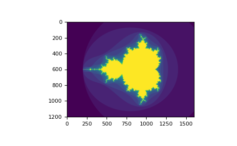
You can look at the following
example to see
how to use boolean indexing to generate an image of the Mandelbrot
set:
>>> import numpy as np
>>> import matplotlib.pyplot as plt
>>> def mandelbrot(h, w, maxit=20, r=2):
...     """Returns an image of the Mandelbrot fractal of size (h,w)."""
...     x = np.linspace(-2.5, 1.5, 4*h+1)
...     y = np.linspace(-1.5, 1.5, 3*w+1)
...     A, B = np.meshgrid(x, y)
...     C = A + B*1j
...     z = np.zeros_like(C)
...     divtime = maxit + np.zeros(z.shape, dtype=int)
...
...     for i in range(maxit):
...         z = z**2 + C
...         diverge = abs(z) > r                    # who is diverging
...         div_now = diverge & (divtime == maxit)  # who is diverging now
...         divtime[div_now] = i                    # note when
...         z[diverge] = r                          # avoid diverging too much
...
...     return divtime
>>> plt.clf()
>>> plt.imshow(mandelbrot(400, 400))
The second way of indexing with booleans is more similar to integer
indexing; for each dimension of the array we give a 1D boolean array
selecting the slices we want:
>>> a = np.arange(12).reshape(3, 4)
>>> b1 = np.array([False, True, True])         # first dim selection
>>> b2 = np.array([True, False, True, False])  # second dim selection
>>>
>>> a[b1, :]                                   # selecting rows
array([[ 4,  5,  6,  7],
       [ 8,  9, 10, 11]])
>>>
>>> a[b1]                                      # same thing
array([[ 4,  5,  6,  7],
       [ 8,  9, 10, 11]])
>>>
>>> a[:, b2]                                   # selecting columns
array([[ 0,  2],
       [ 4,  6],
       [ 8, 10]])
>>>
>>> a[b1, b2]                                  # a weird thing to do
array([ 4, 10])
Note that the length of the 1D boolean array must coincide with the
length of the dimension (or axis) you want to slice. In the previous
example, b1 has length 3 (the number of rows in a), and
b2 (of length 4) is suitable to index the 2nd axis (columns) of
a.
The ix_() function#
The ix_ function can be used to combine different vectors so as to
obtain the result for each n-uplet. For example, if you want to compute
all the a+b*c for all the triplets taken from each of the vectors a, b
and c:
>>> a = np.array([2, 3, 4, 5])
>>> b = np.array([8, 5, 4])
>>> c = np.array([5, 4, 6, 8, 3])
>>> ax, bx, cx = np.ix_(a, b, c)
>>> ax
array([[[2]],

       [[3]],

       [[4]],

       [[5]]])
>>> bx
array([[[8],
        [5],
        [4]]])
>>> cx
array([[[5, 4, 6, 8, 3]]])
>>> ax.shape, bx.shape, cx.shape
((4, 1, 1), (1, 3, 1), (1, 1, 5))
>>> result = ax + bx * cx
>>> result
array([[[42, 34, 50, 66, 26],
        [27, 22, 32, 42, 17],
        [22, 18, 26, 34, 14]],

       [[43, 35, 51, 67, 27],
        [28, 23, 33, 43, 18],
        [23, 19, 27, 35, 15]],

       [[44, 36, 52, 68, 28],
        [29, 24, 34, 44, 19],
        [24, 20, 28, 36, 16]],

       [[45, 37, 53, 69, 29],
        [30, 25, 35, 45, 20],
        [25, 21, 29, 37, 17]]])
>>> result[3, 2, 4]
17
>>> a[3] + b[2] * c[4]
17
You could also implement the reduce as follows:
>>> def ufunc_reduce(ufct, *vectors):
...    vs = np.ix_(*vectors)
...    r = ufct.identity
...    for v in vs:
...        r = ufct(r, v)
...    return r
and then use it as:
>>> ufunc_reduce(np.add, a, b, c)
array([[[15, 14, 16, 18, 13],
        [12, 11, 13, 15, 10],
        [11, 10, 12, 14,  9]],

       [[16, 15, 17, 19, 14],
        [13, 12, 14, 16, 11],
        [12, 11, 13, 15, 10]],

       [[17, 16, 18, 20, 15],
        [14, 13, 15, 17, 12],
        [13, 12, 14, 16, 11]],

       [[18, 17, 19, 21, 16],
        [15, 14, 16, 18, 13],
        [14, 13, 15, 17, 12]]])
The advantage of this version of reduce compared to the normal
ufunc.reduce is that it makes use of the
broadcasting rules
in order to avoid creating an argument array the size of the output
times the number of vectors.
Indexing with strings#
See Structured arrays.
Tricks and Tips#
Here we give a list of short and useful tips.
“Automatic” Reshaping#
To change the dimensions of an array, you can omit one of the sizes
which will then be deduced automatically:
>>> a = np.arange(30)
>>> b = a.reshape((2, -1, 3))  # -1 means "whatever is needed"
>>> b.shape
(2, 5, 3)
>>> b
array([[[ 0,  1,  2],
        [ 3,  4,  5],
        [ 6,  7,  8],
        [ 9, 10, 11],
        [12, 13, 14]],

       [[15, 16, 17],
        [18, 19, 20],
        [21, 22, 23],
        [24, 25, 26],
        [27, 28, 29]]])
Vector Stacking#
How do we construct a 2D array from a list of equally-sized row vectors?
In MATLAB this is quite easy: if x and y are two vectors of the
same length you only need do m=[x;y]. In NumPy this works via the
functions column_stack, dstack, hstack and vstack,
depending on the dimension in which the stacking is to be done. For
example:
>>> x = np.arange(0, 10, 2)
>>> y = np.arange(5)
>>> m = np.vstack([x, y])
>>> m
array([[0, 2, 4, 6, 8],
       [0, 1, 2, 3, 4]])
>>> xy = np.hstack([x, y])
>>> xy
array([0, 2, 4, 6, 8, 0, 1, 2, 3, 4])
The logic behind those functions in more than two dimensions can be
strange.
Histograms#
The NumPy histogram function applied to an array returns a pair of
vectors: the histogram of the array and a vector of the bin edges. Beware:
matplotlib also has a function to build histograms (called hist,
as in Matlab) that differs from the one in NumPy. The main difference is
that pylab.hist plots the histogram automatically, while
numpy.histogram only generates the data.
>>> import numpy as np
>>> rg = np.random.default_rng(1)
>>> import matplotlib.pyplot as plt
>>> # Build a vector of 10000 normal deviates with variance 0.5^2 and mean 2
>>> mu, sigma = 2, 0.5
>>> v = rg.normal(mu, sigma, 10000)
>>> # Plot a normalized histogram with 50 bins
>>> plt.hist(v, bins=50, density=True)       # matplotlib version (plot)
(array...)
>>> # Compute the histogram with numpy and then plot it
>>> (n, bins) = np.histogram(v, bins=50, density=True)  # NumPy version (no plot)
>>> plt.plot(.5 * (bins[1:] + bins[:-1]), n)
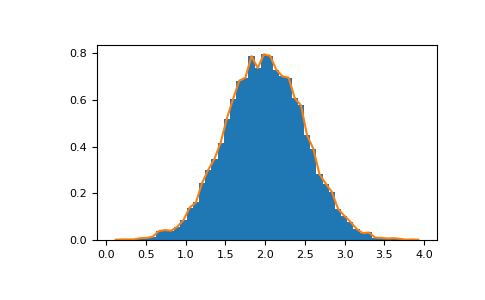
With Matplotlib >=3.4 you can also use plt.stairs(n, bins).
Further reading#
-
The Python tutorial
-
NumPy Reference
-
SciPy Tutorial
-
SciPy Lecture Notes
-
A matlab, R, IDL, NumPy/SciPy dictionary
-
tutorial-svd
#статьи
- 28 окт 2022
-

0
Подробный гайд по самому популярному Python-инструменту для анализа данных и обучения нейронных сетей.
Иллюстрация: A Wolker / Pexels / Colowgee для Skillbox Media

Любитель научной фантастики и технологического прогресса. Хорошо сочетает в себе заумного технаря и утончённого гуманитария. Пишет про IT и радуется этому.
NumPy — это открытая бесплатная Python-библиотека для работы с многомерными массивами, этакий питонячий аналог Matlab. NumPy чаще всего используют в анализе данных и обучении нейронных сетей — в каждой из этих областей нужно проводить много вычислений с такими матрицами.
В этой статье мы собрали всё необходимое для старта работы с этой библиотекой — вам хватит получаса, чтобы разобраться в основных возможностях.
- Базовые функции
- Доступ к элементам
- Создание специальных массивов
- Математические операции
- Копирование и организации
- Дополнительные возможности
Что запомнить
NumPy не просто работает с многомерными массивами, но и делает это быстро. Вообще, интерпретируемые языки производят вычисления медленнее компилируемых, а Python как раз язык интерпретируемый. NumPy же сделана так, чтобы эффективно работать с наборами чисел любого размера в Python.
Библиотека частично написана на Python, а частично на C и C++ — в тех местах, которые требуют скорости. Кроме того, код NumPy оптимизирован под большинство современных процессоров. Кстати, как и у Matlab, для NumPy существуют пакеты, расширяющие её функциональность, — например, библиотека SciPy или Matplotlib.
Инфографика: Оля Ежак для Skillbox Media
Массивы в NumPy отличаются от обычных списков и кортежей в Python тем, что они должны состоять только из элементов одного типа. Такое ограничение позволяет увеличить скорость вычислений в 50 раз, а также избежать ненужных ошибок с приведением и обработкой типов.
Мы установим NumPy через платформу Anaconda, которая содержит много разных библиотек для Python. А ещё покажем, как это сделать через PIP.
NumPy можно также использовать через Jupyter Notebook, Google Colab или другими средствами — как вам удобнее. Поэтому выбирайте любой способ и пойдёмте изучать его.
Сначала надо зайти на официальный сайт Anaconda, чтобы скачать последнюю версию Python и NumPy: есть готовые пакеты под macOS, Windows и Linux.

Скриншот: Skillbox Media
Затем открываем установщик, соглашаемся со всеми пунктами и выбираем место для установки.

Скриншот: Skillbox Media
Чтобы убедиться, что Python точно установился, открываем консоль и вводим туда команду python3 — должен запуститься интерпретатор Python, в котором можно писать код. Выглядит всё это примерно так:
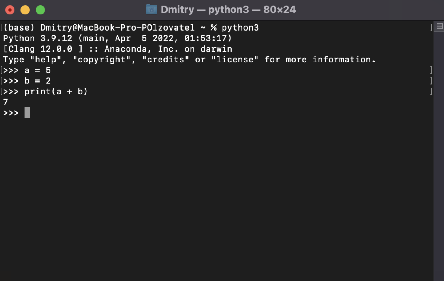
Скриншот: Skillbox Media
Anaconda уже содержит в себе много полезностей — например, NumPy, SciPy, Pandas. Поэтому больше ничего устанавливать не нужно. Достаточно проверить, что библиотека NumPy действительно работает. Введите в интерпретаторе Python в консоли такие команды — пока не важно, что это и как работает, об этом поговорим ниже.
import numpy as np
Следом вот это:
a = np.array ([1,2,3])
А потом выводим значение переменной a — чтобы убедиться, что всё работает:
print (a)
Должно получиться что-то вроде вывода на скриншоте:
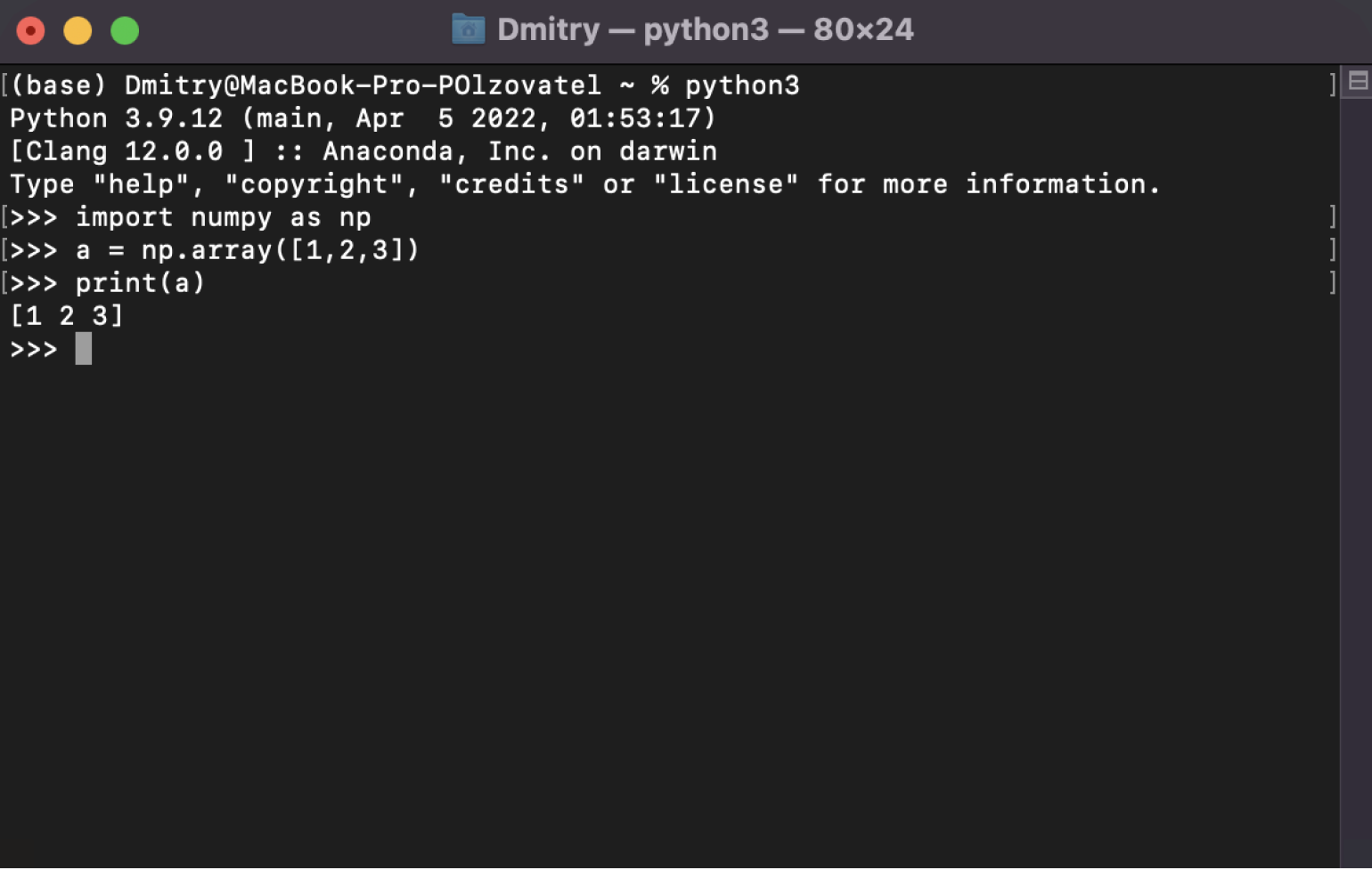
Скриншот: Skillbox Media
Если вам не хочется скачивать огромный пакет Anaconda, вы можете установить только NumPy с помощью встроенного питоновского менеджера пакетов PIP.
Для этого сначала нужно установить Python с официального сайта. Заходим на него, переходим во вкладку Downloads и видим справа последнюю актуальную версию Python:

Скриншот: Skillbox Media
После этого начинается стандартная процедура: выбираем место установки и соглашаемся со всеми пунктами.

В конце нас должны поздравить.

Скриншот: Skillbox Media
Теперь нужно скачать библиотеку NumPy. Открываем консоль и вводим туда команду pip install numpy.
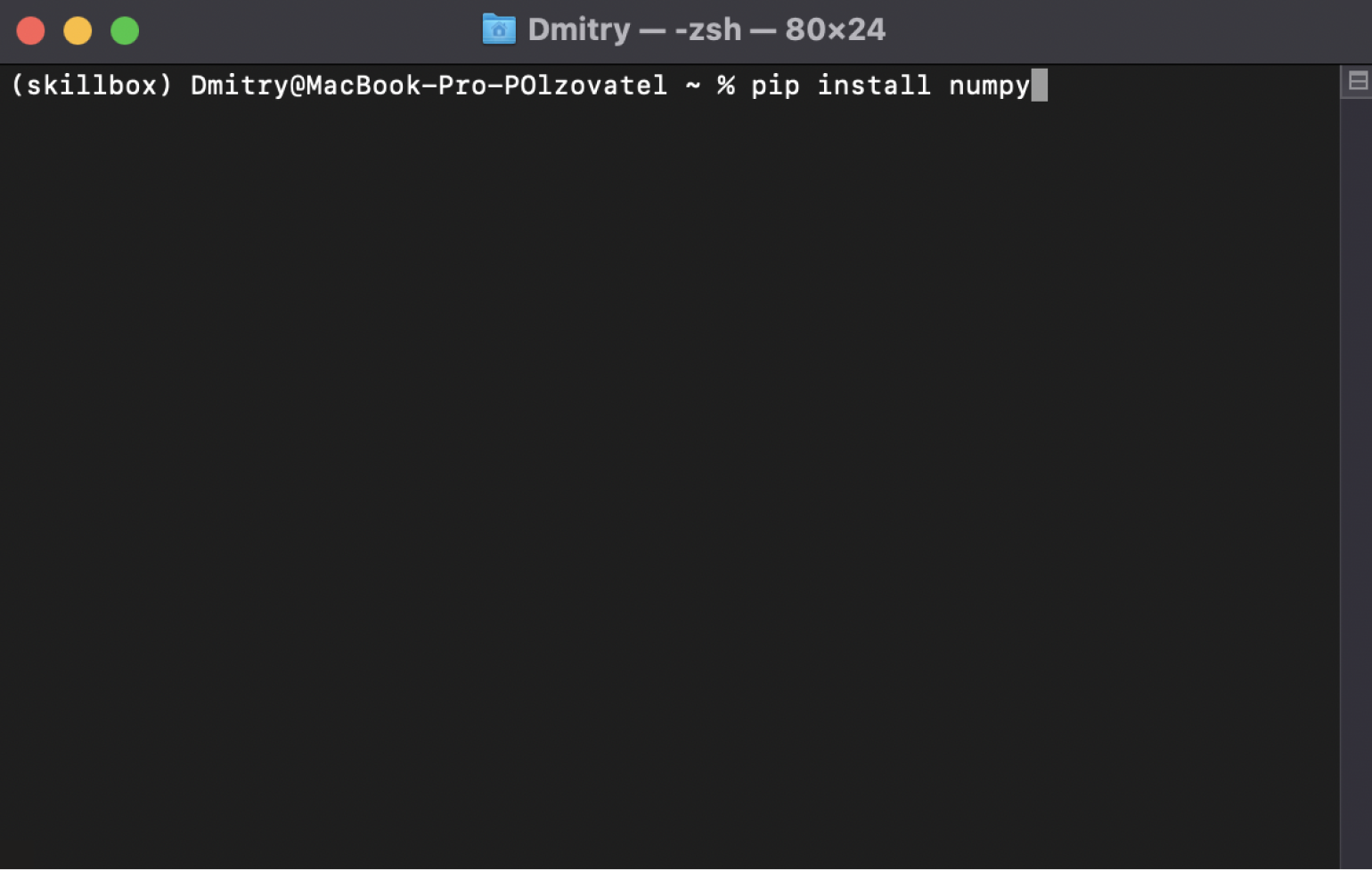
Скриншот: Skillbox Media
Если вдруг у вас выпала ошибка, значит, нужно написать другую похожую команду — pip3 install numpy.
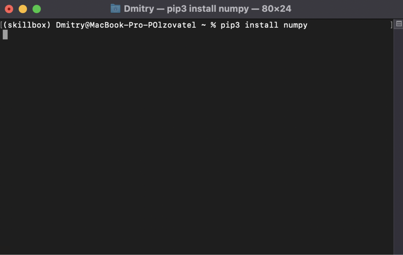
Скриншот: Skillbox Media
Теперь у нас точно должна установиться NumPy. Правда, тут нас уже никто не поздравляет — лишь сухо отмечают, что установка завершилась успешно.
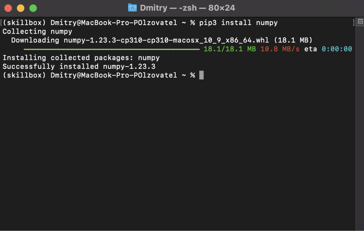
Скриншот: Skillbox Media
Перед тем как использовать NumPy, нужно подключить библиотеку в Python-коде — а вы думали, достаточно установить его? Нет, Python ещё должен узнать, что конкретно в этом проекте NumPy нам нужен.
import numpy as np
np — это уже привычное сокращение для NumPy в Python-сообществе. Оно позволяет быстро обращаться к методам библиотеки (две буквы проще, чем пять). Мы тоже будем придерживаться этого сокращения — мы же профессионалы! Хотя можно использовать NumPy и без присваивания отдельного сокращения или назвать её любыми приятными для вас буквами и символами. Но всё же рекомендуем следовать традициям сообщества, чтобы избежать недопонимания со стороны других программистов.
Теперь приступим к изучению базовых понятий и функций NumPy. А чтобы лучше усвоить изученный материал, рекомендуем внимательно изучать код, самостоятельно переписывать его и поиграться с параметрами и числами.
Главный объект библиотеки NumPy — массив. Создаётся он очень просто:
a = np.array([1, 2, 3])
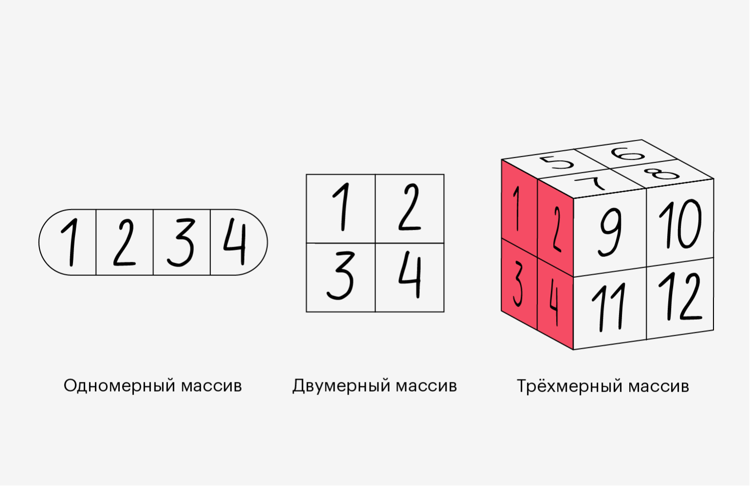
Мы объявили переменную a и использовали встроенную функцию array. В неё нужно положить сам Python-список, который мы хотим создать. Он может быть любой формы: одномерный, двумерный, трёхмерный и так далее. Выше мы создали одномерный массив. Давайте создадим и другие:
a2 = np.array([[1, 2, 3], [4, 5, 6]])
a3 = np.array([[[1, 2, 3], [4, 5, 6]], [[7, 8, 9], [10, 11, 12]]])
Получилось огромное количество скобок. Чтобы понять, как всё это выглядит, воспользуемся функцией print:
print(a)
[1 2 3]

print(a2)
[[1 2 3]
 [4 5 6]]

print(a3)
[[[1 2 3]
  [4 5 6]]

 [[7 8 9]
  [10 11 12]]]
Как мы видим, в первом случае получился двумерный массив, который состоит из двух одномерных. А во втором — трёхмерный, состоящий из двумерных. Если двигаться вверх по измерениям, то они будут следовать похожей логике:
- четырёхмерный массив состоит из трёхмерных;
- пятимерный массив — это несколько четырёхмерных;
- n-мерный массив — это несколько (n-1)-мерных.
Проще показать это на иллюстрации (главное, не потеряйтесь в измерениях):
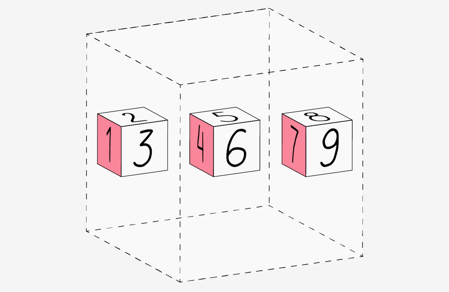
Инфографика: Оля Ежак для Skillbox Media
В NumPy-массивы можно передавать не только целые числа, но и дробные:
b = np.array([1.4, 2.5, 3.7])

print(b)
[1.4 2.5 3.7]
А если вы хотите указать конкретный тип, то это можно сделать с помощью дополнительного параметра dtype:
c = np.array([1, 2, 3], dtype='float32')

print(c)
[1. 2. 3.]
Целые числа сразу были приведены к числам с плавающей точкой. Таких преобразований существует много — они нужны, чтобы не занимать лишнюю память. Например, числа int32 занимают 32 бита, или 4 байта, а int16 — 16 бит, или 2 байта. Программисты используют параметр dtype, когда точно знают, что их переменные будут находиться в диапазоне от −32 768 до 32 767.
Если реальные значения элементов массива выйдут за рамки явно указанного типа, то их значения в какой-то момент просто обнулятся и начнут отсчёт заново:
# Допустим, a — это переменная типа int16, у которой максимальное значение — 32 767

a = 32 000

b = 768
print(a + b)
-32768
Как мы видим, результат обнулился до своего минимального значения — –32 768.
Теперь, когда мы умеем создавать массивы и задавать им разные значения, давайте узнаем, какие у них есть встроенные функции.
Допустим, у нас есть такой объект:
a = np.array([1,2,3], dtype='int32')

print(a)
[1 2 3]
Чтобы узнать, сколько у него измерений, воспользуемся функцией ndim:
print(a.ndim)
1
Всё верно, ведь у нас одномерный массив, или вектор. Если бы он был двумерным, то и результат оказался бы другим:
b = np.array([[1, 2, 3], [4, 5, 6]])

print(b.ndim)
2
Хорошо, с размерностью понятно. А как посчитать количество строк и столбцов? Для этого есть функция shape:
print(a.shape)
(3, )
Получилось слегка странно, но всему есть объяснение. Дело в том, что вектор — это всего лишь одномерный массив. У векторов в библиотеке NumPy есть только строки — или элементы. Поэтому функция shape выдала число 3.
С двумерными массивами ситуация понятнее:
print(b.shape)
(2, 3)
В b — 2 строки и 3 столбца.
Для трёхмерных и n-мерных массивов функция shape будет добавлять дополнительные цифры в кортеже через запятую:
с = np.array([[[1, 2, 3], [4, 5, 6]], [[7, 8, 9], [10, 11, 12]]])

print(c.shape)
(2, 2, 3)
Читается это так: в объекте c два трёхмерных массива с двумя строками и тремя столбцами.
Кроме размерностей, можно также узнать тип элементов — в этом поможет функция dtype (не путайте её с одноимённым параметром):
a = np.array([1,2,3], dtype='int32')

print(a.dtype)
dtype('int32')
Если не присваивать тип элементам вручную, по умолчанию будет задан int32.
Ещё можно узнать количество элементов с помощью функции size:
print(a.size)
3
А через функции itemsize и nbytes можно узнать, какое количество байт в памяти занимает один элемент и какое количество байт занимает весь массив:
b = np.array([[1, 2, 3], [4, 5, 6]], dtype='int16')

print(b.itemsize)
2

print(b.nbytes)
12
Один элемент занимает 2 байта, а весь объект b из 6 элементов — 2 × 6 = 12 байтов.
В NumPy можно обращаться к отдельным элементам, строкам или столбцам, а также точечно выбирать последовательность нужных элементов. Рассмотрим всё подробнее.
Допустим, у нас есть двумерный массив:
a = np.array([[1, 2, 3, 4, 5, 6, 7], [8, 9, 10, 11, 12, 13, 14]])

print(a)
[[ 1  2  3  4  5  6  7]
 [ 8  9 10 11 12 13 14]]
И мы хотим достать их него элемент, который находится в первой строке на пятом месте. Сделать это можно с помощью специального оператора []:
print(a[0, 4])
5
Почему 0 и 4? Потому что нумерация элементов в Python начинается с нуля, а значит, первая строка будет нулевой, а пятый столбец — четвёртым.
Если бы у нас был трёхмерный массив, обращение к его элементам было бы похожим:
c = np.array([[[1, 2, 3], [4, 5, 6]], [[7, 8, 9], [10, 11, 12]]])

print(c)
[[[ 1  2  3]
  [ 4  5  6]]

 [[ 7  8  9]
  [10 11 12]]]

print(c[1, 1, 1])
11
Здесь мы сначала обратились ко второму двумерному массиву, а затем выбрали в нём вторую строку и второй столбец. Там и находилось число 11.
Кроме отдельных элементов, в библиотеке NumPy можно обратиться к целой строке или столбцу с помощью оператора :. Он позволяет выбрать все элементы указанной строки или столбца:
print(a[0, :])
[1 2 3 4 5 6 7]

print(a[:, 0])
[1 8]
В первом случае мы выбрали всю первую строку, а во втором — первый столбец.
Ещё можно использовать продвинутые способы выделения нужных нам элементов.
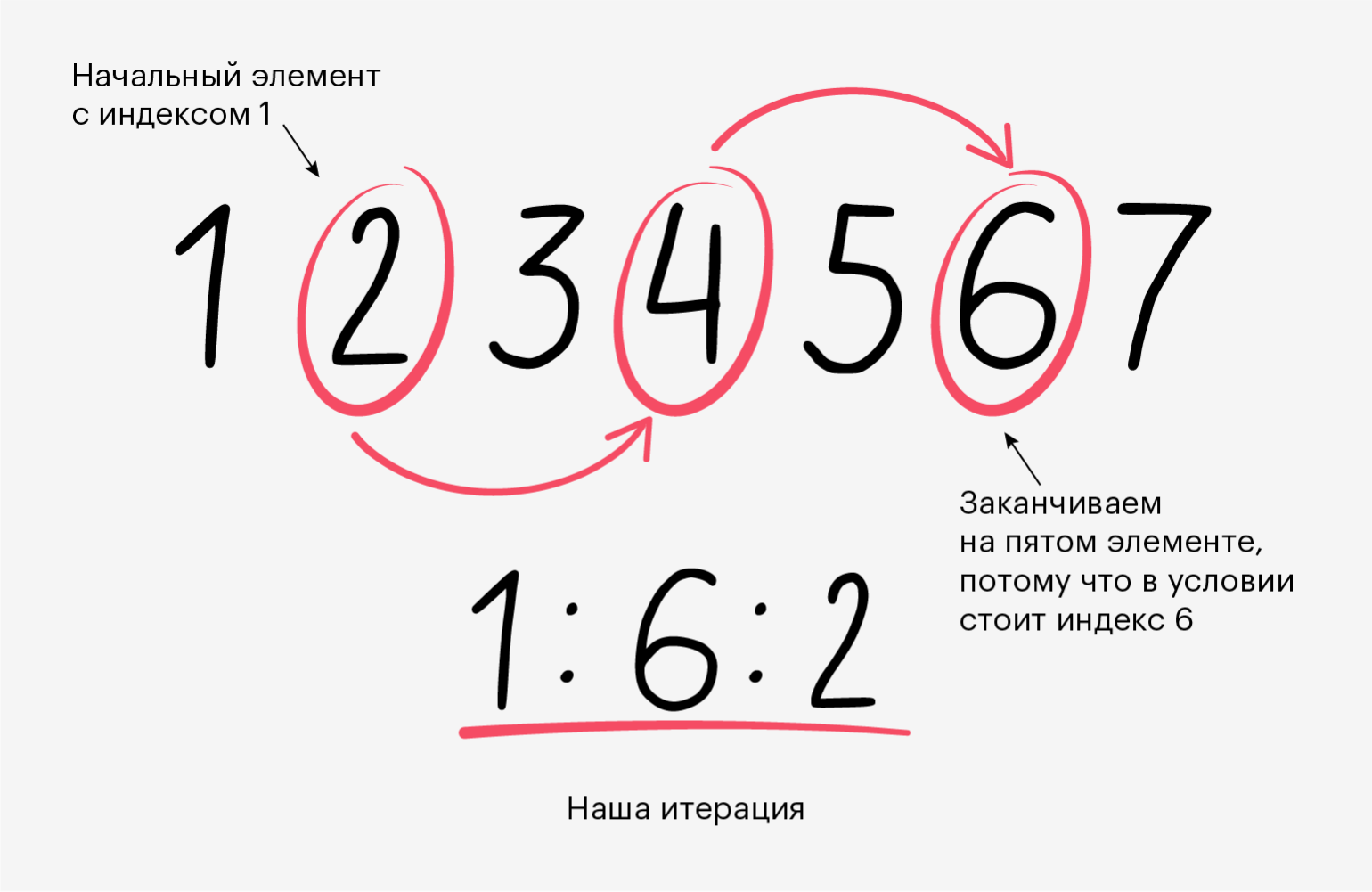
Кстати, оператор : на самом деле представляет собой сокращённую форму конструкции начальный_индекс: конечный_индекс: шаг.
Давайте остановимся на ней подробнее:
b = np.array([[1, 2, 3, 4], [5, 6, 7, 8]])

print(b[0, 1:4:2])
[2 4]
Мы указали, что хотим выбрать первую строку, а затем уточнили, какие именно столбцы нам нужны: 1:4:2.
- Первое число означает, что мы начинаем брать элементы с первого индекса — второго столбца.
- Второе число — что мы заканчиваем итерацию на четвёртом индексе, то есть проходим всю строку.
- Третье число указывает, с каким шагом мы идём по строке. В нашем примере — с шагом в два элемента. То есть мы пройдём по элементам 1, 3 и 5.
Давайте посмотрим на другой пример:
a = np.array([[1, 2, 3, 4, 5, 6, 7], [8, 9, 10, 11, 12, 13, 14]])

print(a)
[[ 1  2  3  4  5  6  7]
 [ 8  9 10 11 12 13 14]]

print(a[1, 0:-1:3])
[8, 11]
Здесь мы использовали отрицательные индексы — они позволяют считать индексы элементов справа налево. –1 означает, что последний индекс — это последний столбец второй строки. Заметьте, что 6-й столбец не вывелся. Это значит, что NumPy не доходит до этого индекса, а заканчивает обход на один индекс раньше.
Инфографика: Оля Ежак для Skillbox Media
Ещё мы можем менять значения в NumPy-массиве с помощью той же операции доступа к элементам. Например:
c = np.array([[0, 2], [4, 6]])
c[0, 0] = 1

print(c)
[[1 2]
 [4 6]]
Мы заменили элемент из первой строки и первого столбца (элемент 0) на единицу. И наш массив успешно изменился.
Кроме отдельных элементов, можно заменять любые последовательности элементов с помощью конструкции начальный_индекс: конечный_индекс: шаг и её упрощённой версии — :.
c = np.array([[0, 2], [4, 6]])
с[0, :] = [3, 3]

print(c)
[[3 3]
 [4 6]]
Теперь в с вся первая строка заменилась на тройки. Главное при такой замене — учитывать размер строки, чтобы не возникло ошибок. Например, если присвоить первой строке вектор из трёх элементов, интерпретатор будет ругаться:
c = np.array([[0, 2], [4, 6]])
c[0, :] = [3, 3, 3]
Traceback (most recent call last):
  File "<stdin>", line 1, in <module>
ValueError: could not broadcast input array from shape (3,) into shape (2,)
Текст ошибки сообщает, что нельзя присвоить одномерному массиву с размером 2 массив размером 3.
Мы научились создавать массивы любой размерности. Но иногда хочется создать их с уже заполненными значениями — например, забить все ячейки нулями или единицами. NumPy может и это.
Массив из нулей. Чтобы создать его, используем функцию zeros.
a = np.zeros((2, 2))

print(a)
[[0. 0.]
 [0. 0.]]
Первое, что нужно помнить, — как задавать размер. Он задаётся кортежем (2, 2). Если указать размер без скобок, то снова получим ошибку:
a = np.zeros(2, 2)
Traceback (most recent call last):
  File "<stdin>", line 1, in <module>
TypeError: Cannot interpret '2' as a data type
А всё потому, что без скобок NumPy расценивает второй элемент (число 2) как тип данных, который должен быть указан для параметра dtype.
Если указать только одно число, создастся вектор размером два элемента. В этом случае уже не нужно ставить дополнительные скобки:
a = np.zeros(2)

print(a)
[0. 0.]
Ещё стоит отметить, что элементам по умолчанию присваивается тип float64. Это дробные числа, которые занимают в памяти 64 бита, или 8 байт. Если нужны именно целые числа, то мы по старой схеме указываем это в параметре dtype — через запятую:
a = np.zeros(2, dtype='int32')

print(a)
[0 0]
Массив из единиц. Он создаётся точно так же, как и из нулей, но используется функция ones:
b = np.ones((4, 2, 2), dtype='int32')
print(b)
[[[1 1]
  [1 1]]

 [[1 1]
  [1 1]]

 [[1 1]
  [1 1]]

 [[1 1]
  [1 1]]]
Здесь мы создали трёхмерный массив из четырёх двумерных, каждый из которых имеет две строки и два столбца. А также указали, что элементы должны иметь тип int32.
Массив из произвольных чисел. Иногда бывает нужно заполнить массив какими-то отличными от нуля и единицы числами. В этом поможет функция full:
c = np.full((2, 2), 5)

print(c)
[[5 5]
 [5 5]]
Здесь мы сначала указали, какой размер должен быть у массива через кортеж, — (2,2), а затем число, которым мы хотим заполнить все его элементы, — 5.
Равно как и у функций zeros и ones, элементы по умолчанию будут иметь тип float64. А размер должен передаваться в виде кортежа — (2, 2).
Массив случайных чисел. Он создаётся с помощью функции random.rand:
d = np.random.rand(3, 2)

print(d)
[[0.76088962 0.14281283]
 [0.32124888 0.34894434]
 [0.66903093 0.72899792]]
Получилось что-то странное. Но так и должно быть — ведь NumPy генерирует случайные числа в диапазоне от 0 до 1 с восемью знаками после запятой.
Ещё одна странность — то, как задаётся размер. Здесь это нужно делать не через кортеж (3, 2), а просто указывая размерности через запятую. Всё потому, что в функции random.rand нет параметра dtype.
Чтобы создать массив случайных чисел, нужно воспользоваться функцией random.randint:
e = np.random.randint(-5, 10, size=(4, 4))

print(e)
[[ 3  1 -4  3]
 [ 0 -2  5  3]
 [ 5 -1  9  2]
 [ 0 -4  9 -2]]
У нас получился массив размером четыре на четыре — size=(4, 4) — с целыми числами из диапазона от –5 до 10. Как и в предыдущем случае, создаётся такой массив слегка странно — но такова жизнь NumPy-программистов.
Единичная матрица. Она нужна тем, кто занимается линейной алгеброй. По диагонали такой матрицы элементы равны единице, а все остальные элементы — нулю. Создаётся она с помощью функции identity или eye:
i = np.identity(4)

print(i)
[[1. 0. 0. 0.]
 [0. 1. 0. 0.]
 [0. 0. 1. 0.]
 [0. 0. 0. 1.]]
Здесь задаётся только количество строк матрицы, потому что единичная матрица должна быть симметричной — иметь одинаковое количество строк и столбцов.
И всё также можно указать тип элементов с помощью параметра dtype:
i = np.identity(4, dtype='int32')

print(i)
[[1 0 0 0]
 [0 1 0 0]
 [0 0 1 0]
 [0 0 0 1]]
Массивы из NumPy поддерживают все стандартные арифметические операции — например, сложение, деление, вычитание. Работает это поэлементно:
a = np.array([1, 2, 3, 4])

print(a)
[1 2 3 4]

print(a + 3)
[4 5 6 7]
К каждому элементу a прибавилось число 3, а размерность не изменилась. Все остальные операции работают точно так же:
print(a - 2)
[-1 0 1 2]

print(a * 2)
[2 4 6 8]

print(a / 2)
[0.5 1. 1.5 2.] #Здесь тип элементов приведён к 'float64'

print(a ** 2)
[1 4 9 16]
Ещё можно проводить любые математические операции с массивами одинакового размера:
a = np.array([[1, 2], [3, 4]])
b = np.array([[2, 2], [2, 2]])

print(a + b)
[[3 4]
 [5 6]]

print(a * b)
[[2 4]
 [6 8]]

print(a ** b)
[[ 1  4]
 [ 9 16]]
Здесь каждый элемент a складывается, умножается и возводится в степень на элемент из такой же позиции массива b.
Кроме примитивных операций, в NumPy можно проводить и более сложные — например, вычислить косинус:
a = np.array([[1, 2], [3, 4]])

print(np.cos(a))
[[ 0.54030231 -0.41614684]
 [-0.9899925  -0.65364362]]
Все математические функции вызываются по похожему шаблону: сначала пишем np.название_математической_функции, а потом передаём внутрь массив — как мы и сделали выше.
Ещё к массивам можно применять различные операции из линейной алгебры, математической статистики и так далее. Давайте для примера перемножим матрицы по правилам линейной алгебры:
a = np.ones((2, 3))

print(a)
[[1. 1. 1.]
 [1. 1. 1.]]

b = np.full((3, 2), 2)
print(b)
[[2 2]
 [2 2]
 [2 2]]

 print(np.matmul(a, b))
[[6. 6.]
 [6. 6.]]
Не будем разбирать математическую составляющую — предполагается, что вы уже знакомы с математикой и используете NumPy для выражения операций языком программирования. Полный список всех поддерживаемых в библиотеке операций можно найти в официальной документации.
Если в NumPy вы присвоите массив другой переменной, то просто создадите ссылку на него. Разберём на примере:
a = np.array([1, 2, 3])
b = a
b[0] = 5

print(b)
[5 2 3]

print(a)
[5 2 3]
Как мы видим, при изменении b меняется также и a. Дело в том, что массивы в NumPy — это только ссылки на области в памяти. Поэтому, когда мы присвоили a переменной b, на самом деле мы просто присвоили ей ссылку на первый элемент a в памяти.
Чтобы создать независимую копию a, используйте функцию copy:
a = np.array([1, 2, 3])
b = a.copy()
b[0] = 5

print(b)
[5 2 3]

print(a)
[1 2 3]
Ещё мы можем менять размер массива с помощью функции reshape:
a = np.array([[1, 2, 3, 4], [5, 6, 7, 8]])

print(a)
[[1 2 3 4]
 [5 6 7 8]]

b = a.reshape((4, 2))

print(b)
[[1 2]
 [3 4]
 [5 6]
 [7 8]]
Изначально размер a был 2 на 4. Мы переделали его под 4 на 2. Заметьте: новые размеры должны соответствовать количеству элементов. В противном случае Python вернет ошибку:
a = np.array([[1, 2, 3, 4], [5, 6, 7, 8]])
b = a.reshape((4, 3))
Traceback (most recent call last):
  File "<stdin>", line 1, in <module>
ValueError: cannot reshape array of size 8 into shape (4,3)
Ещё NumPy позволяет нам «наслаивать» массивы друг на друга и соединять их с помощью функций vstack и hstack:
v1 = np.array([1, 2, 3])
v2 = np.array([9, 8, 7])
v3 = np.vstack([v1, v2])

print(v3)
[[1 2 3]
 [9 8 7]]
Здесь мы создали двумерный массив из двух векторов одинакового размера, которые «поставили» друг на друга. То же самое можно сделать и горизонтально:
h1 = np.ones((2, 4))
h2 = np.zeros((2, 2))
h3 = np.hstack((h1, h2))

print(h3)
[[1. 1. 1. 1. 0. 0.]
 [1. 1. 1. 1. 0. 0.]]
К массиву из единиц справа присоединился массив из нулей. Главное — чтобы количество строк в обоих было одинаковым, иначе вылезет ошибка:
h1 = np.ones((2, 4))
h2 = np.zeros((3, 2))
h3 = np.hstack((h1, h2))
Traceback (most recent call last):
  File "<stdin>", line 1, in <module>
  File "<__array_function__ internals>", line 5, in hstack
  File "/Users/Dmitry/opt/anaconda3/lib/python3.9/site-packages/numpy/core/shape_base.py", line 345, in hstack
    return _nx.concatenate(arrs, 1)
  File "<__array_function__ internals>", line 5, in concatenate
ValueError: all the input array dimensions for the concatenation axis must match exactly, but along dimension 0, the array at index 0 has size 2 and the array at index 1 has size 3
Эта ошибка говорит, что количество строк не совпадает.
NumPy поддерживает другие полезные функции, которые используются реже, но знать о которых полезно. Например, одна из таких функций — чтение файлов с жёсткого диска.
Чтение данных из файла. Допустим, у нас есть файл data.txt с таким содержимым:
1,2,3,5,6,7
8,1,4,2,6,4
9,0,1,7,3,4
Мы можем записать числа в NumPy-массив с помощью функции genfromtxt:
filedata = np.genfromtxt('data.txt', delimiter=',')
filedata = filedata.astype('int32')

print(filedata)
[[1 2 3 5 6 7]
[8 1 4 2 6 4]
[9 0 1 7 3 4]]
Сначала мы достали данные из файла data.txt через функцию genfromtxt. В ней нужно указать считываемый файл, а затем разделитель — чтобы NumPy понимал, где начинаются и заканчиваются числа. У нас разделителем будет ,.
Затем нам нужно привести числа к формату int32 с помощью функции astype, передав в неё нужный нам тип.
Булевы выражения. Ещё одна из возможностей NumPy — булевы выражения для элементов массива. Они позволяют узнать, какие элементы отвечают определённым условиям — например, больше ли каждое число массива 50.
Допустим, у нас есть массив a и мы хотим проверить, действительно ли все его элементы больше 5:
a = np.array([[1, 5, 8], [3, 4, 2]])

print(a > 5)
[[False False  True]
 [False False False]]
На выходе — массив с «ответом» для каждого элемента: больше ли он числа 5. Если меньше или равно, то стоит False, иначе — True.
С помощью булевых выражений можно составлять и более сложные конструкции — например, создавать новые массивы из элементов, которые отвечают определённым условиям:
a = np.array([[1, 5, 8], [3, 4, 2], [2, 6, 7]])

print(a[a > 3])
[5 8 4 6 7]
Мы получили вектор, состоящий из элементов массива a, которые больше трёх.
- NumPy — это библиотека для эффективной работы с массивами любого размера. Она достигает высокой производительности, потому что написана частично на C и C++ и в ней соблюдается принцип локальности — она хранит все элементы последовательно в одном месте.
- Перед тем как использовать NumPy в коде, его нужно подключить с помощью команды import numpy as np.
- Основа NumPy — массив. Чтобы его создать, нужно использовать функцию array и передать туда список в качестве первого аргумента. Вторым аргументом через dtype можно указать тип для всех элементов — например, int16 или float32. По умолчанию для целых чисел указывается int32, а для десятичных — float64.
- Функция ndim позволяет узнать, сколько измерений у массива; shape — его структуру (сколько столбцов и строк); dtype — какой тип у элементов; size — количество элементов; itemsize — сколько байтов занимает один элемент; nbytes — сколько всего памяти занимает массив.
- К элементам массива можно обращаться с помощью оператора [], где указываются индексы нужного элемента. Важно помнить, что индексация начинается с нуля. А ещё в NumPy можно выбирать сразу целые строки или столбцы с помощью оператора : и его продвинутой версии — начальный_индекс: конечный_индекс: шаг.
- Функции zeros, ones, full, random.rand, random.randint, identity и eye помогают быстро создать массивы любого размера с заполненными элементами.
- Все арифметические операции, которые доступны в Python, применимы и к массивам NumPy. Главное — помнить, что операции проводятся поэлементно. А для сложных операций, таких как вычисление производной, также есть свои функции.
- NumPy-массивы нельзя просто присвоить другой переменной, чтобы скопировать. Для этого существует функция copy. А чтобы поменять структуру данных, можно применить функции reshape, vstack и hstack.
- Ещё в NumPy есть дополнительные функции — например, чтение из файла с помощью genfromtxt и булевы выражения, которые позволяют выбирать элементы из набора данных по заданным условиям.

Научитесь: Профессия Data Scientist
Узнать больше
Время на прочтение
19 мин
Количество просмотров 234K
 NumPy — это расширение языка Python, добавляющее поддержку больших многомерных массивов и матриц, вместе с большой библиотекой высокоуровневых математических функций для операций с этими массивами.
Первая часть учебника рассказывает об основах работы с NumPy: создании массивов, их атрибутах, базовых операциях, поэлементном применении функций, индексах, срезах, итерировании. Рассматриваются различные манипуляции с преобразованием формы массива, объединение массивов из нескольких и наоборот — разбиение одного на несколько более мелких. В конце мы обсудим поверхностное и глубокое копирование.
Основы
Если вы еще не устанавливали NumPy, то взять его можно здесь. Используемая версия Python — 2.6.
Основным объектом NumPy является однородный многомерный массив. Это таблица элементов (обычно чисел), всех одного типа, индексированных последовательностями натуральных чисел.
Под «многомерностью» массива мы понимаем то, что у него может быть несколько измерений или осей. Поскольку слово «измерение» является неоднозначным, вместо него мы чаще будем использовать слова «ось» (axis) и «оси» (axes). Число осей называется рангом (rank).
Например, координаты точки в трехмерном пространстве [1, 2, 1] это массив ранга 1 у него есть только одна ось. Длина этой оси — 3. Другой пример, массив
[[ 1., 0., 0.],

 [ 0., 1., 2.]]
представляет массив ранга 2 (то есть это двухмерный массив). Длина первого измерения (оси) — 2, длина второй оси — 3. Для получения дополнительной информации смотрите глоссарий Numpy.
Класс многомерных массивов называется ndarray. Заметим, что это не то же самое, что класс array стандартной библиотеки Python, который используется только для одномерных массивов. Наиболее важные атрибуты объектов ndarray:
ndarray.ndim — число осей (измерений) массива. Как уже было сказано, в мире Python число измерений часто называют рангом.
ndarray.shape — размеры массива, его форма. Это кортеж натуральных чисел, показывающий длину массива по каждой оси. Для матрицы из n строк и m столбов, shape будет (n,m). Число элементов кортежа shape равно рангу массива, то есть ndim.
ndarray.size — число всех элементов массива. Равно произведению всех элементов атрибута shape.
ndarray.dtype — объект, описывающий тип элементов массива. Можно определить dtype, используя стандартные типы данных Python. NumPy здесь предоставляет целый букет возможностей, например: bool_, character, int_, int8, int16, int32, int64, float_, float8, float16, float32, float64, complex_, complex64, object_.
ndarray.itemsize — размер каждого элемента массива в байтах. Например, для массива из элементов типа float64 значение itemsize равно 8 (=64/8), а для complex32 этот атрибут равен 4 (=32/8).
ndarray.data — буфер, содержащий фактические элементы массива. Обычно нам не будет нужно использовать этот атрибут, потому как мы будем обращаться к элементам массива с помощью индексов.
Пример
Определим следующий массив:
Copy Source | Copy HTML<br/>>>> from numpy import *<br/>>>> a = arange(10).reshape(2,5)<br/>>>> a<br/>array([[ 0, 1, 2, 3, 4],<br/> [5, 6, 7, 8, 9]]) <br/>
Мы только что создали объект массива с именем a. У массива a есть несколько атрибутов или свойств. В Python атрибуты отдельного объекта обозначаются как name_of_object.attribute. В нашем случае:
a.shapeэто (2,5)a.ndimэто 2 (что равно длинеa.shape)a.sizeэто 10a.dtype.nameэто int32a.itemsizeэто 4, что означает, что int32 занимает 4 байта памяти.
Вы можете проверить все эти атрибуты, просто набрав их в интерактивном режиме:
Copy Source | Copy HTML<br/>>>> a.shape<br/>(2, 5)<br/>>>> a.dtype.name<br/>'int32' <br/>
И так далее.
Создание массивов
Есть много способов для того, чтобы создать массив. Например, вы можете создать массив из обычных списков или кортежей Python, используя функцию array():
Copy Source | Copy HTML<br/>>>> from numpy import *<br/>>>> a = array( [2,3,4] )<br/>>>> a<br/>array([2, 3, 4])<br/>>>> type(a)<br/><type 'numpy.ndarray'> <br/>
Функция array() трансформирует вложенные последовательности в многомерные массивы. Тип массива зависит от типа элементов исходной последовательности.
Copy Source | Copy HTML<br/>>>> b = array( [ (1.5,2,3), (4,5,6) ] ) # это станет массивом float элементов<br/>>>> b<br/>array([[ 1.5, 2. , 3. ],<br/> [ 4. , 5. , 6. ]]) <br/>
Раз у нас есть массив, мы можем взглянуть на его атрибуты:
Copy Source | Copy HTML<br/>>>> b.ndim # число осей<br/>2<br/>>>> b.shape # размеры<br/>(2, 3)<br/>>>> b.dtype # тип (8-байтовый float)<br/>dtype('float64')<br/>>>> b.itemsize # размер элемента данного типа<br/>8 <br/>
Тип массива может быть явно указан в момент создания:
Copy Source | Copy HTML<br/>>>> c = array( [ [1,2], [3,4] ], dtype=complex )<br/>>>> c<br/>array([[ 1.+ 0.j, 2.+ 0.j],<br/> [ 3.+ 0.j, 4.+ 0.j]]) <br/>
Часто встречающаяся ошибка состоит в вызове функции array() с множеством числовых аргументов вместо предполагаемого единственного аргумента в виде списка чисел:
Copy Source | Copy HTML<br/>>>> a = array(1,2,3,4) # WRONG<br/>>>> a = array([1,2,3,4]) # RIGHT <br/>
Функция array() не единственная функция для создания массивов. Обычно элементы массива вначале неизвестны, а массив, в котором они будут храниться уже нужен. Поэтому имеется несколько функций для того, чтобы создавать массивы с каким-то исходным содержимым. По умолчанию тип создаваемого массива — float64.
Функция zeros() создает массив нулей, а функция ones() — массив единиц:
Copy Source | Copy HTML<br/>>>> zeros( (3,4) ) # аргумент задает форму массива<br/>array([[ 0., 0., 0., 0.],<br/> [ 0., 0., 0., 0.],<br/> [ 0., 0., 0., 0.]])<br/>>>> ones( (2,3,4), dtype=int16 ) # то есть также может быть задан dtype<br/>array([[[ 1, 1, 1, 1],<br/> [ 1, 1, 1, 1],<br/> [ 1, 1, 1, 1]],<br/> [[ 1, 1, 1, 1],<br/> [ 1, 1, 1, 1],<br/> [ 1, 1, 1, 1]]], dtype=int16) <br/>
Функция empty() создает массив без его заполнения. Исходное содержимое случайно и зависит от состояния памяти на момент создания массива (то есть от того мусора, что в ней хранится):
Copy Source | Copy HTML<br/>>>> empty( (2,3) )<br/>array([[ 3.73603959e-262, 6.02658058e-154, 6.55490914e-260],<br/> [ 5.30498948e-313, 3.14673309e-307, 1.00000000e+000]])<br/>>>> empty( (2,3) ) # содержимое меняется при новом вызове<br/>array([[ 3.14678735e-307, 6.02658058e-154, 6.55490914e-260],<br/> [ 5.30498948e-313, 3.73603967e-262, 8.70018275e-313]]) <br/>
Для создания последовательностей чисел, в NumPy имеется функция, аналогичная range(), только вместо списков она возвращает массивы:
Copy Source | Copy HTML<br/>>> arange( 10, 30, 5 )<br/>array([10, 15, 20, 25])<br/>>>> arange( 0, 2, 0.3 )<br/>array([ 0. , 0.3, 0.6, 0.9, 1.2, 1.5, 1.8]) <br/>
При использовании arange() с аргументами типа float, сложно быть уверенным в том, сколько элементов будет получено (из-за ограничения точности чисел с плавающей запятой). Поэтому, в таких случаях обычно лучше использовать функцию linspace() которая вместо шага в качестве одного из аргументов принимает число, равное количеству нужных элементов:
Copy Source | Copy HTML<br/>>>> linspace( 0, 2, 9 ) # 9 чисел от 0 до 2<br/>array([ 0. , 0.25, 0.5 , 0.75, 1. , 1.25, 1.5 , 1.75, 2. ])<br/>>>> x = linspace( 0, 2*pi, 100 ) # полезно для вычисления значений функции в множестве точек<br/>>>> f = sin(x) <br/>
Печать массивов
Когда вы печатаете массив, NumPy показывает их схожим с вложенными списками образом, но размещает немного иначе:
- последняя ось печатается слева направо,
- предпоследняя — сверху вниз,
- и оставшиеся — также сверху вниз, разделяя пустой строкй.
Одномерные массивы выводятся как строки, двухмерные — как матрицы, а трехмерные — как списки матриц.
Copy Source | Copy HTML<br/>>>> a = arange(6) # 1d array<br/>>>> print a<br/>[0 1 2 3 4 5]<br/>>>><br/>>>> b = arange(12).reshape(4,3) # 2d array<br/>>>> print b<br/>[[ 0 1 2]<br/> [ 3 4 5]<br/> [ 6 7 8]<br/> [ 9 10 11]]<br/>>>><br/>>>> c = arange(24).reshape(2,3,4) # 3d array<br/>>>> print c<br/>[[[ 0 1 2 3]<br/> [ 4 5 6 7]<br/> [ 8 9 10 11]]<br/> [[12 13 14 15]<br/> [16 17 18 19]<br/> [20 21 22 23]]] <br/>
Если массив слишком большой, чтобы его печатать, NumPy автоматически скрывает центральную часть массива и выводит только его уголки:
Copy Source | Copy HTML<br/>>>> print arange(10000)<br/>[ 0 1 2 ..., 9997 9998 9999]<br/>>>><br/>>>> print arange(10000).reshape(100,100)<br/>[[ 0 1 2 ..., 97 98 99]<br/> [ 100 101 102 ..., 197 198 199]<br/> [ 200 201 202 ..., 297 298 299]<br/> ...,<br/> [9700 9701 9702 ..., 9797 9798 9799]<br/> [9800 9801 9802 ..., 9897 9898 9899]<br/> [9900 9901 9902 ..., 9997 9998 9999]] <br/>
Если вам действительно нужно увидеть все, что происходит в большом массиве, выведя его полностью, используйте функцию установки печати set_printoptions():
Copy Source | Copy HTML<br/>>>> set_printoptions(threshold=nan) <br/>
Базовые операции
Арифметические операции над массивами выполняются поэлементно. Создается новый массив, который заполняется результатами действия оператора.
Copy Source | Copy HTML<br/>>>> a = array( [20,30,40,50] )<br/>>>> b = arange( 4 )<br/>>>> c = a-b<br/>>>> c<br/>array([20, 29, 38, 47])<br/>>>> b**2<br/>array([ 0, 1, 4, 9])<br/>>>> 10*sin(a)<br/>array([ 9.12945251, -9.88031624, 7.4511316 , -2.62374854])<br/>>>> a<35<br/>array([True, True, False, False], dtype=bool) <br/>
В отличие от матричного подхода, оператор произведения * в массивах NumPy работает также поэлементно. Матричное произведение может быть осуществлено либо функцией dot(), либо созданием объектов матриц, которое будет рассмотрено далее (во второй части пособия).
Copy Source | Copy HTML<br/>>>> A = array( [[1,1],<br/>... [ 0,1]] )<br/>>>> B = array( [[2, 0],<br/>... [3,4]] )<br/>>>> A*B # поэлементное произведение<br/>array([[2, 0],<br/> [ 0, 4]])<br/>>>> dot(A,B) # матричное произведение<br/>array([[5, 4],<br/> [3, 4]]) <br/>
Некоторые операции делаются «на месте», без создания нового массива.
Copy Source | Copy HTML<br/>>>> a = ones((2,3), dtype=int)<br/>>>> b = random.random((2,3))<br/>>>> a *= 3<br/>>>> a<br/>array([[3, 3, 3],<br/> [3, 3, 3]])<br/>>>> b += a<br/>>>> b<br/>array([[ 3.69092703, 3.8324276 , 3.0114541 ],<br/> [ 3.18679111, 3.3039349 , 3.37600289]])<br/>>>> a += b # b конвертируется к типу int<br/>>>> a<br/>array([[6, 6, 6],<br/> [6, 6, 6]]) <br/>
При работе с массивами разных типов, тип результирующего массива соответствует более общему или более точному типу.
Copy Source | Copy HTML<br/>>>> a = ones(3, dtype=int32)<br/>>>> b = linspace( 0,pi,3)<br/>>>> b.dtype.name<br/>'float64'<br/>>>> c = a+b<br/>>>> c<br/>array([ 1. , 2.57079633, 4.14159265])<br/>>>> c.dtype.name<br/>'float64'<br/>>>> d = exp(c*1j)<br/>>>> d<br/>array([ 0.54030231+ 0.84147098j, - 0.84147098+ 0.54030231j,<br/> - 0.54030231- 0.84147098j])<br/>>>> d.dtype.name<br/>'complex128' <br/>
Многие унарные операции, такие как вычисление суммы всех элементов массива, представлены в виде методов класса ndarray.
Copy Source | Copy HTML<br/>>>> a = random.random((2,3))<br/>>>> a<br/>array([[ 0.6903007 , 0.39168346, 0.16524769],<br/> [ 0.48819875, 0.77188505, 0.94792155]])<br/>>>> a.sum()<br/>3.4552372100521485<br/>>>> a.min()<br/> 0.16524768654743593<br/>>>> a.max()<br/> 0.9479215542670073 <br/>
По умолчанию, эти операции применяются к массиву, как если бы он был списком чисел, независимо от его формы. Однако, указав параметр axis можно применить операцию по указанной оси массива:
Copy Source | Copy HTML<br/>>>> b = arange(12).reshape(3,4)<br/>>>> b<br/>array([[ 0, 1, 2, 3],<br/> [ 4, 5, 6, 7],<br/> [ 8, 9, 10, 11]])<br/>>>><br/>>>> b.sum(axis= 0) # сумма в каждом столбце<br/>array([12, 15, 18, 21])<br/>>>><br/>>>> b.min(axis=1) # наименьшее число в каждой строке<br/>array([ 0, 4, 8])<br/>>>><br/>>>> b.cumsum(axis=1) # накопительная сумма каждой строки<br/>array([[ 0, 1, 3, 6],<br/> [ 4, 9, 15, 22],<br/> [ 8, 17, 27, 38]]) <br/>
Универсальные функции
NumPy обеспечивает работу с известными математическими функциями sin, cos, exp и так далее. Но в NumPy эти функции называются универсальными (ufunc). Причина присвоения такого имени кроется в том, что в NumPy эти функции работают с массивами также поэлементно, и на выходе получается массив значений.
Copy Source | Copy HTML<br/>>>> B = arange(3)<br/>>>> B<br/>array([ 0, 1, 2])<br/>>>> exp(B)<br/>array([ 1. , 2.71828183, 7.3890561 ])<br/>>>> sqrt(B)<br/>array([ 0. , 1. , 1.41421356])<br/>>>> C = array([2., -1., 4.])<br/>>>> add(B, C)<br/>array([ 2., 0., 6.]) <br/>
Индексы, срезы, итерации
Одномерные массивы осуществляют операции индексирования, срезов и итераций очень схожим образом с обычными списками и другими последовательностями Python.
Copy Source | Copy HTML<br/>>>> a = arange(10)**3<br/>>>> a<br/>array([ 0, 1, 8, 27, 64, 125, 216, 343, 512, 729])<br/>>>> a[2]<br/>8<br/>>>> a[2:5]<br/>array([ 8, 27, 64])<br/>>>> a[:6:2] = -1000 # изменить элементы в a<br/>>>> a<br/>array([-1000, 1, -1000, 27. -1000, 125, 216, 343, 512, 729])<br/>>>> a[::-1] # перевернуть a<br/>array([ 729, 512, 343, 216, 125, -1000, 27, -1000, 1, -1000])<br/>>>> for i in a:<br/>... print i**(1/3.),<br/>...<br/>nan 1. 0 nan 3. 0 nan 5.0 6.0 7.0 8.0 9. 0 <br/>
У многомерных массивов на каждую ось приходится один индекс. Индексы передаются в виде последовательности чисел, разделенных запятыми:
Copy Source | Copy HTML<br/>>>> def f(x,y):<br/>... return 10*x+y<br/>...<br/>>>> b = fromfunction(f,(5,4),dtype=int)<br/>>>> b<br/>array([[ 0, 1, 2, 3],<br/> [10, 11, 12, 13],<br/> [20, 21, 22, 23],<br/> [30, 31, 32, 33],<br/> [40, 41, 42, 43]])<br/>>>> b[2,3]<br/>23<br/>>>> b[:,1] # второй столбец массива b<br/>array([ 1, 11, 21, 31, 41])<br/>>>> b[1:3,:] # вторая и третья строки массива b<br/>array([[10, 11, 12, 13],<br/> [20, 21, 22, 23]]) <br/>
Когда индексов меньше, чем осей, отсутствующие индексы предполагаются дополненными с помощью срезов:
Copy Source | Copy HTML<br/>>>> b[-1] # последняя строка. Эквивалентно b[-1,:]<br/>array([40, 41, 42, 43]) <br/>
b[i] можно читать как b[i, <столько символов ':', сколько нужно>]. В NumPy это также может быть записано с помощью точек, как b[i, ...].
Например, если x имеет ранг 5 (то есть у него 5 осей), тогда
x[1, 2, ...]эквивалентноx[1, 2, :, :, :],x[... , 3]то же самое, чтоx[:, :, :, :, 3]иx[4, ... , 5, :]этоx[4, :, :, 5, :].
Copy Source | Copy HTML<br/>>>> c = array( [ [[ 0, 1, 2], # 3d array<br/>... [ 10, 12, 13]],<br/>...<br/>... [[100,101,102],<br/>... [110,112,113]] ] )<br/>>>> c.shape<br/>(2, 2, 3)<br/>>>> c[1,...] # то же, что c[1,:,:] или c[1]<br/>array([[100, 101, 102],<br/> [110, 112, 113]])<br/>>>> c[...,2] # то же, что c[:,:,2]<br/>array([[ 2, 13],<br/> [102, 113]]) <br/>
Итерирование многомерных массивов начинается с первой оси:
Copy Source | Copy HTML<br/>>>> for row in b:<br/>... print row<br/>...<br/>[0 1 2 3]<br/>[10 11 12 13]<br/>[20 21 22 23]<br/>[30 31 32 33]<br/>[40 41 42 43] <br/>
Однако, если нужно перебрать поэлементно весь массив, как если бы он был одномерным, для этого можно использовать атрибут flat:
Copy Source | Copy HTML<br/>>>> for element in b.flat:<br/>... print element,<br/>...<br/>0 1 2 3 10 11 12 13 20 21 22 23 30 31 32 33 40 41 42 43 <br/>
Манипуляции с формой
Как уже говорилось, у массива есть форма (shape), определяемая числом элементов вдоль каждой оси:
Copy Source | Copy HTML<br/>>>> a = floor(10*random.random((3,4)))<br/>>>> a<br/>array([[ 7., 5., 9., 3.],<br/> [ 7., 2., 7., 8.],<br/> [ 6., 8., 3., 2.]])<br/>>>> a.shape<br/>(3, 4) <br/>
Форма массива может быть изменена с помощью различных команд:
Copy Source | Copy HTML<br/>>>> a.ravel() # делает массив плоским<br/>array([ 7., 5., 9., 3., 7., 2., 7., 8., 6., 8., 3., 2.])<br/>>>> a.shape = (6, 2)<br/>>>> a.transpose()<br/>array([[ 7., 9., 7., 7., 6., 3.],<br/> [ 5., 3., 2., 8., 8., 2.]]) <br/>
Порядок элементов в массиве в результате функции ravel() соответствует обычному «C-стилю», то есть, чем правее индекс, тем он «быстрее изменяется»: за элементом a[0,0] следует a[0,1]. Если одна форма массива была изменена на другую, массив переформировывается также в «C-стиле». В таком порядке NumPy обычно и создает массивы, так что для функции ravel() обычно не требуется копировать аргумент, но если массив был создан из срезов другого массива, копия может потребоваться. Функции ravel() и reshape() также могут работать (при использовании дополнительного аргумента) в FORTRAN-стиле, в котором быстрее изменяется более левый индекс.
Функция reshape() возвращает ее аргумент с измененной формой, в то время как метод resize() изменяет сам массив:
Copy Source | Copy HTML<br/>>>> a<br/>array([[ 7., 5.],<br/> [ 9., 3.],<br/> [ 7., 2.],<br/> [ 7., 8.],<br/> [ 6., 8.],<br/> [ 3., 2.]])<br/>>>> a.resize((2,6))<br/>>>> a<br/>array([[ 7., 5., 9., 3., 7., 2.],<br/> [ 7., 8., 6., 8., 3., 2.]]) <br/>
Если при операции такой перестройки один из аргументов задается как -1, то он автоматически рассчитывается в соответствии с остальными заданными:
Copy Source | Copy HTML<br/>>>> a.reshape(3,-1)<br/>array([[ 7., 5., 9., 3.],<br/> [ 7., 2., 7., 8.],<br/> [ 6., 8., 3., 2.]]) <br/>
Объединение массивов
Несколько массивов могут быть объединены вместе вдоль разных осей:
Copy Source | Copy HTML<br/>>>> a = floor(10*random.random((2,2)))<br/>>>> a<br/>array([[ 1., 1.],<br/> [ 5., 8.]])<br/>>>> b = floor(10*random.random((2,2)))<br/>>>> b<br/>array([[ 3., 3.],<br/> [ 6., 0.]])<br/>>>> vstack((a,b))<br/>array([[ 1., 1.],<br/> [ 5., 8.],<br/> [ 3., 3.],<br/> [ 6., 0.]])<br/>>>> hstack((a,b))<br/>array([[ 1., 1., 3., 3.],<br/> [ 5., 8., 6., 0.]]) <br/>
Функция column_stack() объединяет одномерные массивы в качестве столбцов двумерного массива:
Copy Source | Copy HTML<br/>>>> column_stack((a,b))<br/>array([[ 1., 1., 3., 3.],<br/> [ 5., 8., 6., 0.]])<br/>>>> a=array([4.,2.])<br/>>>> b=array([2.,8.])<br/>>>> a[:,newaxis] # Это дает нам 2D-ветор<br/>array([[ 4.],<br/> [ 2.]])<br/>>>> column_stack((a[:,newaxis],b[:,newaxis]))<br/>array([[ 4., 2.],<br/> [ 2., 8.]])<br/>>>> vstack((a[:,newaxis],b[:,newaxis])) # Поведение vstack другое<br/>array([[ 4.],<br/> [ 2.],<br/> [ 2.],<br/> [ 8.]]) <br/>
Аналогично для строк имеется функция row_stack(). Для массивов с более, чем двумя осями, hstack() объединяет массивы по первым осям, vstack() — по последним, дополнительные аргументы позволяют задать число осей по которым должно произойти объединение.
В сложных случаях, могут быть полезны r_[] и с_[], позволяющие создавать одномерные массивы, с помощью последовательностей чисел вдоль одной оси. В них также имеется возможность использовать «:» для задания диапазона литералов:
Copy Source | Copy HTML<br/>>>> r_[1:4, 0,4]<br/>array([1, 2, 3, 0, 4]) <br/>
Разделение одного массива на несколько более мелких
Используя hsplit() вы можете разбить массив вдоль горизонтальной оси, указав либо число возвращаемых массивов одинаковой формы, либо номера столбцов, после которых массив разрезается ножницами:
Copy Source | Copy HTML<br/>>>> a = floor(10*random.random((2,12)))<br/>>>> a<br/>array([[ 8., 8., 3., 9., 0., 4., 3., 0., 0., 6., 4., 4.],<br/> [ 0., 3., 2., 9., 6., 0., 4., 5., 7., 5., 1., 4.]])<br/>>>> hsplit(a,3) # Разбить на 3 массива<br/>[array([[ 8., 8., 3., 9.],<br/> [ 0., 3., 2., 9.]]), array([[ 0., 4., 3., 0.],<br/> [ 6., 0., 4., 5.]]), array([[ 0., 6., 4., 4.],<br/> [ 7., 5., 1., 4.]])]<br/>>>> hsplit(a,(3,4)) # Разрезать a после третьего и четвертого столбца<br/>[array([[ 8., 8., 3.],<br/> [ 0., 3., 2.]]), array([[ 9.],<br/> [ 9.]]), array([[ 0., 4., 3., 0., 0., 6., 4., 4.],<br/> [ 6., 0., 4., 5., 7., 5., 1., 4.]])] <br/>
Функция vsplit() разбивает массив вдоль вертикальной оси, а array_split() позволяет указать оси, вдоль которых произойдет разбиение.
Копии и представления
При работе с массивами, их данные иногда необходимо копировать в другой массив, а иногда нет. Это часто является источником путаницы среди новичков. Возможно всего три случая:
Вообще никаких копий
Простое присваивание не создает ни копии массива, ни копии его данных:
Copy Source | Copy HTML<br/>>>> a = arange(12)<br/>>>> b = a # никакого нового объекта создано не было<br/>>>> b is a # a и b это два имени для одного объекта ndarray <br/>True<br/>>>> b.shape = 3,4 # изменит форму a<br/>>>> a.shape<br/>(3, 4) <br/>
Python передает изменяемые объекты как ссылки, поэтому вызовы функций также не создают копий:
Copy Source | Copy HTML<br/>>>> def f(x):<br/>... print id(x)<br/>...<br/>>>> id(a)<br/>148293216<br/>>>> f(a)<br/>148293216 <br/>
Представление или поверхностная копия
Разные объекты массивов могут использовать одни и те же данные. Метод view() создает новый объект массива, являющийся представлением тех же данных.
Copy Source | Copy HTML<br/>>>> c = a.view()<br/>>>> c is a<br/>False<br/>>>> c.base is a # c это представление данных, принадлежащих a<br/>True<br/>>>> c.flags.owndata<br/>False<br/>>>><br/>>>> c.shape = 2,6 # форма а не поменяется<br/>>>> a.shape<br/>(3, 4)<br/>>>> c[ 0,4] = 1234 # данные а изменятся<br/>>>> a<br/>array([[ 0, 1, 2, 3],<br/> [1234, 5, 6, 7],<br/> [ 8, 9, 10, 11]]) <br/>
Срез массива это представление:
Copy Source | Copy HTML<br/>>>> s = a[:,1:3]<br/>>>> s[:] = 10 # s[:] это представление s. Заметьте разницу между s=10 и s[:]=10<br/>>>> a<br/>array([[ 0, 10, 10, 3],<br/> [1234, 10, 10, 7],<br/> [ 8, 10, 10, 11]]) <br/>
Глубокая копия
Метод copy() создает настоящую копию массива и его данных:
Copy Source | Copy HTML<br/>>>> d = a.copy() # создается новый объект массива с новыми данными<br/>>>> d is a<br/>False<br/>>>> d.base is a # d не имеет ничего общего с а<br/>False<br/>>>> d[ 0, 0] = 9999<br/>>>> a<br/>array([[ 0, 10, 10, 3],<br/> [1234, 10, 10, 7],<br/> [ 8, 10, 10, 11]]) <br/>
В заключение
Итак, в первой части мы рассмотрели самые важные базовые операции работы с массивами. В дополнение к этой части, я советую хорошую шпаргалку. Во второй части мы поговорим о более специфических вещах: об индексировании с помощью массивов индексов или булевых величин, реализации операций линейной алгебры и классе matrix и разных полезных трюках.
Пакет NumPy является незаменимым помощником Python. Он тянет на себе анализ данных, машинное обучение и научные вычисления, а также существенно облегчает обработку векторов и матриц. Некоторые ведущие пакеты Python используют NumPy как основной элемент своей инфраструктуры. К их числу относятся scikit-learn, SciPy, pandas и tensorflow. Помимо возможности разобрать по косточкам числовые данные, умение работать с NumPy дает значительное преимущество при отладке более сложных сценариев библиотек.
Содержание
- Создание массивов NumPy
- Арифметические операции над массивами NumPy
- Индексация массива NumPy
- Агрегирование в NumPy
- Создание матриц NumPy на примерах
- Арифметические операции над матрицами NumPy
- dot() Скалярное произведение NumPy
- Индексация матрицы NumPy
- Агрегирование матриц NumPy
- Транспонирование и изменение формы матриц в numpy
- Примеры работы с NumPy
- Таблицы NumPy — примеры использования таблиц
- Аудио и временные ряды в NumPy
- Обработка изображений в NumPy
- Обработка текста в NumPy на примерах
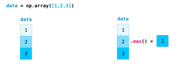
В данной статье будут рассмотрены основные способы использования NumPy на примерах, а также типы представления данных (таблицы, картинки, текст и так далее) перед их последующей подачей модели машинного обучения.
Можно создать массив NumPy (он же ndarray), передав ему список Python, используя np.array(). В данном случае Python создает массив, который выглядит следующим образом:
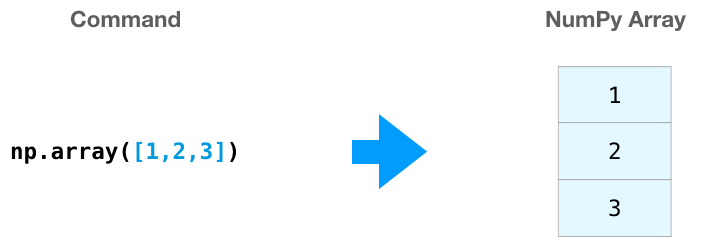
Нередки случаи, когда необходимо, чтобы NumPy инициализировал значения массива.
Есть вопросы по Python?
На нашем форуме вы можете задать любой вопрос и получить ответ от всего нашего сообщества!
Telegram Чат & Канал
Вступите в наш дружный чат по Python и начните общение с единомышленниками! Станьте частью большого сообщества!
Паблик VK
Одно из самых больших сообществ по Python в социальной сети ВК. Видео уроки и книги для вас!
Для этого NumPy использует такие методы, как ones(), zeros() и random.random(). Требуется просто передать им количество элементов, которые необходимо сгенерировать:
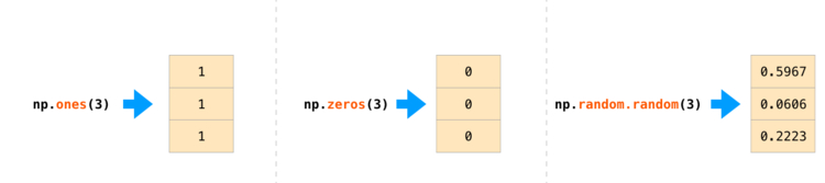
После создания массивов можно манипулировать ими довольно любопытными способами.
Арифметические операции над массивами NumPy
Создадим два массива NumPy и продемонстрируем выгоду их использования.
Массивы будут называться data и ones:
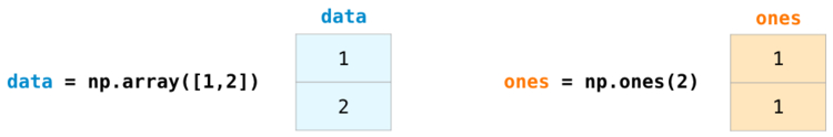
При сложении массивов складываются значения каждого ряда. Это сделать очень просто, достаточно написать data + ones:
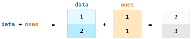
Новичкам может прийтись по душе тот факт, что использование абстракций подобного рода не требует написания циклов for с вычислениями. Это отличная абстракция, которая позволяет оценить поставленную задачу на более высоком уровне.
Помимо сложения, здесь также можно выполнить следующие простые арифметические операции:
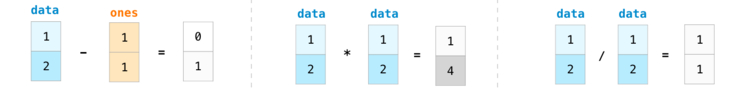
Довольно часто требуется выполнить какую-то арифметическую операцию между массивом и простым числом. Ее также можно назвать операцией между вектором и скалярной величиной. К примеру, предположим, в массиве указано расстояние в милях, и его нужно перевести в километры. Для этого нужно выполнить операцию data * 1.6:
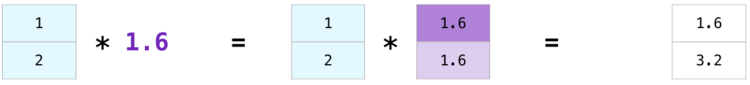
Как можно увидеть в примере выше, NumPy сам понял, что умножить на указанное число нужно каждый элемент массива. Данный концепт называется трансляцией, или broadcating. Трансляция бывает весьма полезна.
Индексация массива NumPy
Массив NumPy можно разделить на части и присвоить им индексы. Принцип работы похож на то, как это происходит со списками Python.
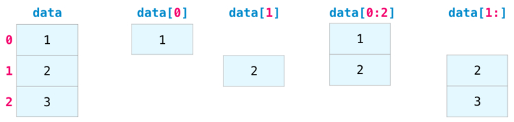
Агрегирование в NumPy
Дополнительным преимуществом NumPy является наличие в нем функций агрегирования:
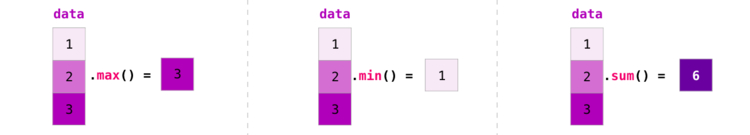
Функциями min(), max() и sum() дело не ограничивается.
К примеру:
mean()позволяет получить среднее арифметическое;prod()выдает результат умножения всех элементов;stdнужно для среднеквадратического отклонения.
Это лишь небольшая часть довольно обширного списка функций агрегирования в NumPy.
Использование нескольких размерностей NumPy
Все перечисленные выше примеры касаются векторов одной размерности. Главным преимуществом NumPy является его способность использовать отмеченные операции с любым количеством размерностей.
Создание матриц NumPy на примерах
Созданные в следующей форме списки из списков Python можно передать NumPy. Он создаст матрицу, которая будет представлять данные списки:
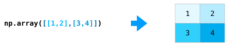
Упомянутые ранее методы ones(), zeros() и random.random() можно использовать так долго, как того требует проект.
Достаточно только добавить им кортеж, в котором будут указаны размерности матрицы, которую мы создаем.
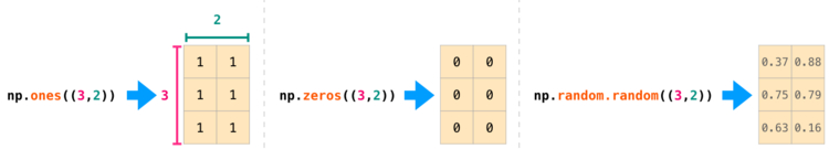
Арифметические операции над матрицами NumPy
Матрицы можно складывать и умножать при помощи арифметических операторов (+ - * /). Стоит, однако, помнить, что матрицы должны быть одного и того же размера. NumPy в данном случае использует операции координат:
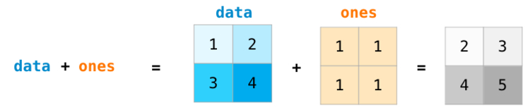
Арифметические операции над матрицами разных размеров возможны в том случае, если размерность одной из матриц равно одному. Это значит, что в матрице только один столбец или один ряд. В таком случае для выполнения операции NumPy будет использовать правила трансляции:
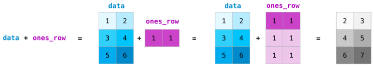
dot() Скалярное произведение NumPy
Главное различие с обычными арифметическими операциями здесь в том, что при умножении матриц используется скалярное произведение. В NumPy каждая матрица может использовать метод dot(). Он применяется для проведения скалярных операций с рассматриваемыми матрицами:
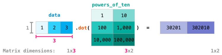
На изображении выше под каждой фигурой указана ее размерность. Это сделано с целью отметить, что размерности обеих матриц должны совпадать с той стороны, где они соприкасаются. Визуально представить данную операцию можно следующим образом:
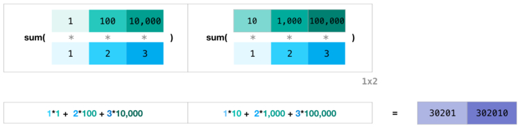
Индексация матрицы NumPy
Операции индексации и деления незаменимы, когда дело доходит до манипуляции с матрицами:
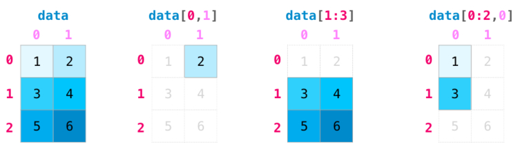
Агрегирование матриц NumPy
Агрегирование матриц происходит точно так же, как агрегирование векторов:
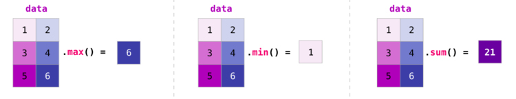
Используя параметр axis, можно агрегировать не только все значения внутри матрицы, но и значения за столбцами или рядами.
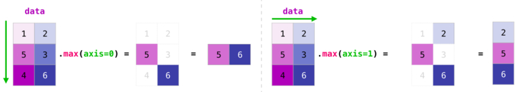
Транспонирование и изменение формы матриц в numpy
Нередки случаи, когда нужно повернуть матрицу. Это может потребоваться при вычислении скалярного произведения двух матриц. Тогда возникает необходимость наличия совпадающих размерностей. У массивов NumPy есть полезное свойство под названием T, что отвечает за транспонирование матрицы.
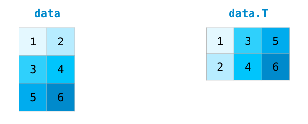
Некоторые более сложные ситуации требуют возможности переключения между размерностями рассматриваемой матрицы. Это типично для приложений с машинным обучением, где некая модель может запросить определенную форму вывода, которая является отличной от формы начального набора данных. В таких ситуациях пригодится метод reshape() из NumPy. Здесь от вас требуется только передать новые размерности для матрицы. Для размерности вы можете передать -1, и NumPy выведет ее верное значение, опираясь на данные рассматриваемой матрицы:
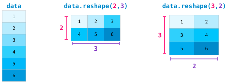
Еще больше размерностей NumPy
NumPy может произвести все вышеперечисленные операции для любого количества размерностей. Структура данных, расположенных центрально, называется ndarray, или n-мерным массивом.
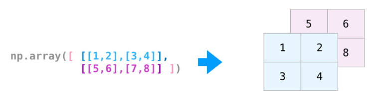
В большинстве случаев для указания новой размерности требуется просто добавить запятую к параметрам функции NumPy:
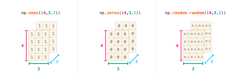
На заметку: Стоит иметь в виду, что при выводе 3-мерного массива NumPy результат, представленный в виде текста, выглядит иначе, нежели показано в примере выше. Порядок вывода n-мерного массива NumPy следующий — последняя ось зацикливается быстрее всего, а первая медленнее всего. Это значит, что вывод
np.ones((4,3,2))будет иметь вид:
|
array([[[1., 1.], [1., 1.], [1., 1.]], [[1., 1.], [1., 1.], [1., 1.]], [[1., 1.], [1., 1.], [1., 1.]], [[1., 1.], [1., 1.], [1., 1.]]]) |
Примеры работы с NumPy
Подытожим все вышесказанное. Вот несколько примеров полезных инструментов NumPy, которые могут значительно облегчить процесс написания кода.
Математические формулы NumPy
Необходимость внедрения математических формул, которые будут работать с матрицами и векторами, является главной причиной использования NumPy. Именно поэтому NumPy пользуется большой популярностью среди представителей науки. В качестве примера рассмотрим формулу среднеквадратичной ошибки, которая является центральной для контролируемых моделей машинного обучения, что решают проблемы регрессии:
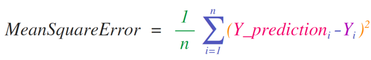
Реализовать данную формулу в NumPy довольно легко:
![]()
Главное достоинство NumPy в том, что его не заботит, если predictions и labels содержат одно или тысячи значение (до тех пор, пока они оба одного размера). Рассмотрим пример, последовательно изучив четыре операции в следующей строке кода:
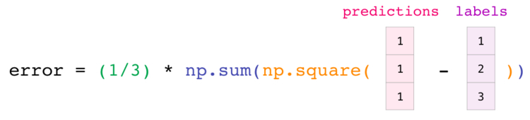
У обоих векторов predictions и labels по три значения. Это значит, что в данном случае n равно трем. После выполнения указанного выше вычитания мы получим значения, которые будут выглядеть следующим образом:
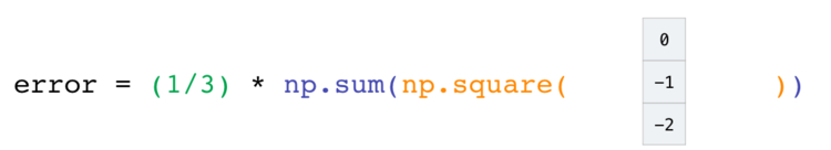
Затем мы можем возвести значения вектора в квадрат:
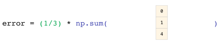
Теперь мы вычисляем эти значения:
Таким образом мы получаем значение ошибки некого прогноза и score за качество модели.
Представление данных NumPy
Задумайтесь о всех тех типах данных, которыми вам понадобится оперировать, создавая различные модели работы (электронные таблицы, изображения, аудио и так далее). Очень многие типы могут быть представлены как n-мерные массивы:
Таблицы NumPy — примеры использования таблиц
Таблица значений является двумерной матрицей. Каждый лист таблицы может быть отдельной переменной. Для работы с таблицами в Python чаще всего используется pandas.DataFrame, что задействует NumPy и строит поверх него.
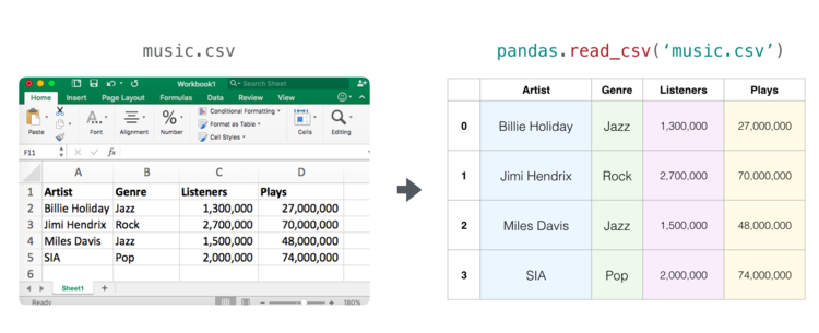
Аудио и временные ряды в NumPy
По сути аудио файл — это одномерный массив семплов. Каждый семпл представляет собой число, которое является крошечным фрагментов аудио сигнала. Аудио CD-качества может содержать 44 100 семплов в секунду, каждый из которых является целым числом в промежутке между -32767 и 32768. Это значит, что десятисекундный WAVE-файл CD-качества можно поместить в массив NumPy длиной в 10 * 44 100 = 441 000 семплов.
Хотите извлечь первую секунду аудио? Просто загрузите файл в массив NumPy под названием audio, после чего получите audio[: 44100].
Фрагмент аудио файла выглядит следующим образом:
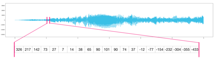
То же самое касается данных временных рядов, например, изменения стоимости акций со временем.
Обработка изображений в NumPy
Изображение является матрицей пикселей по размеру (высота х ширина).
Если изображение черно-белое, то есть представленное в полутонах, каждый пиксель может быть представлен как единственное число. Обычно между 0 (черный) и 255 (белый). Хотите обрезать квадрат размером 10 х 10 пикселей в верхнем левом углу картинки? Просто попросите в NumPy image[:10, :10].
Вот как выглядит фрагмент изображения:
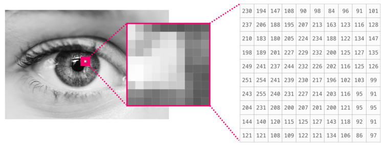
Если изображение цветное, каждый пиксель представлен тремя числами. Здесь за основу берется цветовая модель RGB — красный (R), зеленый (G) и синий (B).
В данном случае нам понадобится третья размерность, так как каждая клетка вмещает только одно число. Таким образом, цветная картинка будет представлена массивом ndarray с размерностями: (высота х ширина х 3).

Обработка текста в NumPy на примерах
Когда дело доходит до текста, подход несколько меняется. Цифровое представление текста предполагает создание некого python словаря, то есть инвентаря всех уникальных слов, которые бы распознавались моделью, а также векторно (embedding step). Попробуем представить в цифровой форме цитату из стихотворения арабского поэта Антара ибн Шаддада, переведенную на английский язык:
“Have the bards who preceded me left any theme unsung?”
Перед переводом данного предложения в нужную цифровую форму модель должна будет проанализировать огромное количество текста. Здесь можно обработать небольшой набор данный, после чего использовать его для создания словаря из 71 290 слов.
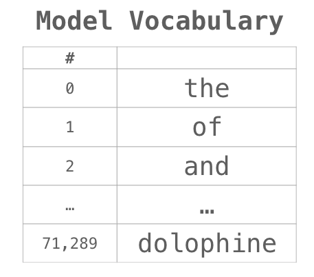
Предложение может быть разбито на массив токенов, что будут словами или частями слов в зависимости от установленных общих правил:
![]()
Затем в данной таблице словаря вместо каждого слова мы ставим его id:
![]()
Однако данные id все еще не обладают достаточным количеством информации о модели как таковой. Поэтому перед передачей последовательности слов в модель токены/слова должны быть заменены их векторными представлениями. В данном случае используется 50-мерное векторное представление Word2vec.
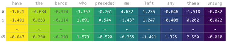
Здесь ясно видно, что у массива NumPy есть несколько размерностей [embedding_dimension x sequence_length]. На практике все выглядит несколько иначе, однако данное визуальное представление более понятно для разъяснения общих принципов работы.
Для лучшей производительности модели глубокого обучения обычно сохраняют первую размерность для пакета. Это происходит из-за того, что тренировка модели происходит быстрее, если несколько примеров проходят тренировку параллельно. Здесь особенно полезным будет reshape(). Например, такая модель, как BERT, будет ожидать ввода в форме: [batch_size, sequence_length, embedding_size].
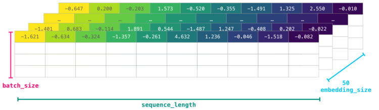
Теперь мы получили числовой том, с которым модель может работать и делать полезные вещи. Некоторые строки остались пустыми, однако они могут быть заполнены другими примерами, на которых модель может тренироваться или делать прогнозы.
(На заметку: Поэма, строчку из которой мы использовали в примере, увековечила своего автора в веках. Будучи незаконнорожденным сыном главы племени от рабыни, Антара ибн Шаддан мастерски владел языком поэзии. Вокруг исторической фигуры поэта сложились мифы и легенды, а его стихи стали частью классической арабской литературы).

Являюсь администратором нескольких порталов по обучению языков программирования Python, Golang и Kotlin. В составе небольшой команды единомышленников, мы занимаемся популяризацией языков программирования на русскоязычную аудиторию. Большая часть статей была адаптирована нами на русский язык и распространяется бесплатно.
E-mail: vasile.buldumac@ati.utm.md
Образование
Universitatea Tehnică a Moldovei (utm.md)
- 2014 — 2018 Технический Университет Молдовы, ИТ-Инженер. Тема дипломной работы «Автоматизация покупки и продажи криптовалюты используя технический анализ»
- 2018 — 2020 Технический Университет Молдовы, Магистр, Магистерская диссертация «Идентификация человека в киберпространстве по фотографии лица»
Перевод
Ссылка на автора

Мир работает на данных, и каждый должен знать, как с ними работать.
Трудно представить современный, технически грамотный бизнес, который не использует анализ данных, науку о данных, машинное обучение или искусственный интеллект в той или иной форме. NumPy лежит в основе всех этих областей.
Хотя невозможно точно знать, сколько людей учатся анализировать данные и работать с ними, вполне можно предположить, что десятки тысяч (если не миллионы) людей должны понимать NumPy и как его использовать. Из-за этого я потратил последние три месяца на то, чтобы составить, как я надеюсь, лучшее вводное руководство по NumPy!Если есть что-то, что вы хотите увидеть в этом руководстве, пожалуйста, оставьте примечание в комментариях или обращайтесь в любое время!
Если вы новичок в анализе данных, этот для вас.

Руководство абсолютного новичка по NumPy

Добро пожаловать в NumPy!
NumPy (NumericalPython) — это библиотека Python с открытым исходным кодом, которая используется практически во всех областях науки и техники. Это универсальный стандарт для работы с числовыми данными в Python, и он лежит в основе научных экосистем Python и PyData. В число пользователей NumPy входят все — от начинающих программистов до опытных исследователей, занимающихся самыми современными научными и промышленными исследованиями и разработками. API-интерфейс NumPy широко используется в пакетах Pandas, SciPy, Matplotlib, scikit-learn, scikit-image и в большинстве других научных и научных пакетов Python.
Библиотека NumPy содержит многомерный массив и матричные структуры данных (дополнительную информацию об этом вы найдете в следующих разделах). Он предоставляет ndarray, однородный объект n-мерного массива, с методами для эффективной работы с ним. NumPy может использоваться для выполнения самых разнообразных математических операций над массивами. Он добавляет мощные структуры данных в Python, которые гарантируют эффективные вычисления с массивами и матрицами, и предоставляет огромную библиотеку математических функций высокого уровня, которые работают с этими массивами и матрицами.
Узнайте больше о NumPy здесь!
Установка NumPy
Чтобы установить NumPy, я настоятельно рекомендую использовать научный дистрибутив Python. Если вам нужны полные инструкции по установке NumPy в вашей операционной системе, вы можете найти все детали здесь,
Если у вас уже есть Python, вы можете установить NumPy с помощью
conda install numpy
или
pip install numpy
Если у вас еще нет Python, вы можете рассмотреть возможность использования анаконда, Это самый простой способ начать. Преимущество этого дистрибутива в том, что вам не нужно слишком беспокоиться об отдельной установке NumPy или каких-либо основных пакетов, которые вы будете использовать для анализа данных, таких как pandas, Scikit-Learn и т. Д.
Если вам нужна более подробная информация об установке, вы можете найти всю информацию об установке на scipy.org,

Если у вас возникли проблемы с установкой Anaconda, вы можете ознакомиться с этой статьей:
Как успешно установить Anaconda на Mac (и на самом деле заставить его работать)
Краткое и безболезненное руководство по правильной установке Anaconda и исправлению страшной ошибки «команда conda not found»
towardsdatascience.com
Как импортировать NumPy
Каждый раз, когда вы хотите использовать пакет или библиотеку в своем коде, вам сначала нужно сделать его доступным.
Чтобы начать использовать NumPy и все функции, доступные в NumPy, вам необходимо импортировать его. Это можно легко сделать с помощью этого оператора импорта:
import numpy as np
(Мы сокращаем «numpy» до «np», чтобы сэкономить время и сохранить стандартизированный код, чтобы любой, кто работает с вашим кодом, мог легко его понять и запустить.)
В чем разница между списком Python и массивом NumPy?
NumPy предоставляет вам огромный выбор быстрых и эффективных числовых опций. Хотя список Python может содержать разные типы данных в одном списке, все элементы в массиве NumPy должны быть однородными. Математические операции, которые должны выполняться над массивами, были бы невозможны, если бы они не были однородными.
Зачем использовать NumPy?

Массивы NumPy быстрее и компактнее, чем списки Python. Массив потребляет меньше памяти и намного удобнее в использовании. NumPy использует гораздо меньше памяти для хранения данных и предоставляет механизм задания типов данных, который позволяет оптимизировать код еще дальше.
Что такое массив?
Массив является центральной структурой данных библиотеки NumPy. Это таблица значений, которая содержит информацию о необработанных данных, о том, как найти элемент и как интерпретировать элемент. Он имеет сетку элементов, которые можно проиндексировать в различные способы Все элементы имеют одинаковый тип, называемыймассив dtype(тип данных).
Массив может быть проиндексирован набором неотрицательных целых чисел, логическими значениями, другим массивом или целыми числами.рангмассива это количество измерений.формамассива — это кортеж целых чисел, дающий размер массива по каждому измерению.
Одним из способов инициализации массивов NumPy является использование вложенных списков Python.
a = np.array([[1 , 2, 3, 4], [5, 6, 7, 8], [9, 10, 11, 12]])
Мы можем получить доступ к элементам в массиве, используя квадратные скобки. Когда вы получаете доступ к элементам, помните, чтоиндексирование в NumPy начинается с 0, Это означает, что если вы хотите получить доступ к первому элементу в вашем массиве, вы получите доступ к элементу «0».
print(a[0])
Выход:
[1 2 3 4]
Больше информации о массивах
1D array, 2D array, ndarray, vector, matrix
Иногда вы можете услышать массив, называемый «ndarray», что означает «N-мерный массив. »N-мерный массив — это просто массив с любым количеством измерений. Вы также можете услышать1-Дили одномерный массив,2-Дили двумерный массив и т. д. Класс NumPy ndarray используется для представления как матриц, так и векторов.вектормассив с одним столбцом, в то время какматрицассылается на массив с несколькими столбцами.
Каковы атрибуты массива?
Массив обычно представляет собой контейнер с фиксированным размером элементов одного типа и размера. Количество измерений и элементов в массиве определяется его формой. Форма массива — это набор неотрицательных целых чисел, которые определяют размеры каждого измерения.
В NumPy размеры называютсяоси, Это означает, что если у вас есть 2D-массив, который выглядит так:
[[0., 0., 0.],
 [1., 1., 1.]]
Ваш массив имеет 2 оси. Первая ось имеет длину 2, а вторая ось имеет длину 3.
Как и в других объектах-контейнерах Python, к содержимому массива можно получить доступ и изменить его, проиндексировав или разделив массив. Разные массивы могут совместно использовать одни и те же данные, поэтому изменения, внесенные в один массив, могут быть видны в другом.
Атрибуты массива отражают информацию, присущую самому массиву. Если вам нужно получить или даже установить свойства массива без создания нового массива, вы часто можете получить доступ к массиву через его атрибуты.
Узнайте больше об атрибутах массива здесь и узнать о массив объектов здесь,
Как создать базовый массив
np.array()
np.zeros()
np.ones()
np.empty()
np.arange()
np.linspace()
dtype
Чтобы создать массив NumPy, вы можете использовать функциюnp.array (),
Все, что вам нужно сделать, чтобы создать простой массив, это передать ему список. При желании вы также можете указать тип данных в вашем списке. Вы можете найти больше информации о типах данных здесь,
import numpy as npa = np.array([1, 2, 3])
Вы можете визуализировать ваш массив следующим образом:

Помимо создания массива из последовательности элементов, вы можете легко создать массив, заполненный0s:
Входные данные:
np.zeros(2)
Выход:
array([0., 0.])
Или массив заполнен1s:
Входные данные:
np.ones(2)
Выход:
array([1., 1.])
Или дажеопорожнитьмассив! Функцияопорожнитьсоздает массив, исходное содержимое которого является случайным и зависит от состояния памяти.
Входные данные:
# Create an empty array with 2 elements
np.empty(2)
Вы можете создать массив с диапазоном элементов:
Входные данные:
np.arange(4)
Выход:
array([0, 1, 2, 3])
И даже массив, который содержит диапазон равномерно распределенных интервалов. Для этого вам нужно будет указатьпервыйколичество,прошлойномер, аразмер шага,
Входные данные:
np.arange(2,9,2)
Выход:
array([2, 4, 6, 8])
Вы также можете использоватьnp.linspace ()создать массив со значениями, которые расположены линейно в заданном интервале:
Входные данные:
np.linspace(0,10,5)
Выход:
array([ 0. , 2.5, 5. , 7.5, 10. ])
Указание вашего типа данных
Хотя тип данных по умолчанию — с плавающей запятой (float64), вы можете явно указать, какой тип данных вы хотите использовать, используя dtype.
Входные данные:
array = np.ones(2, dtype=int)
array
Выход:
array([1, 1])
Узнайте больше о создании массивов здесь,

Добавление, удаление и сортировка элементов
np.append()
np.delete()
np.sort()
Если вы начнете с этого массива:
arr = np.array([1, 2, 3, 4, 5, 6, 7, 8])
Вы можете добавлять элементы в свой массив в любое время с помощьюnp.append (), Обязательно укажите массив и элементы, которые вы хотите включить.
Входные данные:
np.append(arr, [1,2])
Выход:
array([1, 2, 3, 4, 5, 6, 7, 8, 1, 2])
Вы можете удалить элемент сnp.delete (), Если вы хотите удалить элемент в позиции 1 вашего массива, вы можете запустить:
Входные данные:
np.delete(arr, 1)
Выход:
array([1, 3, 4, 5, 6, 7, 8])
Подробнее о добавлении массива читайте здесь а также удаляя элементы здесь,
Сортировка элемента проста сnp.sort (), Вы можете указать ось, вид и порядок при вызове функции. Подробнее о сортировке массива читайте здесь,
Если вы начнете с этого массива:
arr = np.array([2, 1, 5, 3, 7, 4, 6, 8])
Вы можете быстро отсортировать числа в порядке возрастания с помощью:
Входные данные:
np.sort(arr)
Выход:
array([1, 2, 3, 4, 5, 6, 7, 8])
В дополнение к sort, который возвращает отсортированную копию массива, вы можете использовать:argsort, который является непрямая сортировка по указанной оси,lexsort, который является непрямая стабильная сортировка по нескольким ключам,searchsorted, который будет найти элементы в отсортированном массиве, а такжераздел, который является частичная сортировка,
Как вы знаете форму и размер массива?
ndarray.ndim()
ndarray.size()
ndarray.shape()
ndarray ndimскажет вам количество осей или размеров массива.
ndarray.sizeскажет вам общее количество элементов массива. Этопродуктэлементов формы массива.
ndarray.shapeбудет отображать кортеж целых чисел, которые указывают количество элементов, хранящихся вдоль каждого измерения массива. Если, например, у вас есть 2D-массив с 2 строками и 3 столбцами, форма вашего массива будет (2,3).
Например, если вы создаете этот массив:
array_example = np.array([[[0, 1, 2, 3]
                           [4, 5, 6, 7]],                           [[0, 1, 2, 3]
                            [4, 5, 6, 7]],                            [0 ,1 ,2, 3]
                            [4, 5, 6, 7]]])
Чтобы узнать количество измерений массива, запустите:
Входные данные:
array_example.ndim
Выход:
3
Чтобы найти общее количество элементов в массиве, запустите:
Входные данные:
array_example.size
Выход:
24
И чтобы найти форму вашего массива, запустите:
Входные данные:
array_example.shape
Выход:
(3,2,4)
Подробнее о размерах здесь, размер здесь, а также формировать здесь,
Можете ли вы изменить форму массива?
np.reshape()
Да!
С помощьюnp.reshape ()придаст массиву новую форму без изменения данных. Просто помните, что когда вы используете метод reshape, массив, который вы хотите создать, должен иметь то же количество элементов, что и исходный массив. Если вы начинаете с массива из 12 элементов, вам нужно убедиться, что ваш новый массив также содержит в общей сложности 12 элементов.
Если вы начнете с этого массива:
a = np.arange(6)
print(a)
Выход:
[0 1 2 3 4 5]
Вы можете использоватьИзменение формы ()изменить свой массив. Например, вы можете изменить этот массив в массив с тремя строками и двумя столбцами:
Входные данные:
b = a.reshape(3,2)
print(b)
Выход:
[[0 1]
 [2 3]
 [4 5]]
Сnp.reshapeВы можете указать несколько дополнительных параметров:
Входные данные:
numpy.reshape(a, newshape, order)
это массив, который будет изменен.
newshapeэто новая форма, которую вы хотите. Вы можете указать целое число или кортеж целых чисел. Если вы укажете целое число, результатом будет массив этой длины. Форма должна быть совместима с оригинальной формой.
приказ: «C» означает чтение / запись элементов с использованием C-подобного порядка индексов, «F» означает чтение / запись элементов с использованием Fortran-подобного порядка индексов, «A» означает чтение / запись элементов в Fortran-подобном индексе порядок, если a является непрерывным в памяти Fortran, C-подобный порядок в противном случае. (Это необязательный параметр, указывать его не нужно.)
Узнайте больше о манипуляции с формой здесь,
Как преобразовать одномерный массив в двухмерный массив (как добавить новую ось в массив)
np.newaxis
np.expand_dims
Вы можете использоватьnp.newaxisа такжеnp.expand_dimsувеличить размеры вашего существующего массива.
С помощьюnp.newaxisувеличит размеры вашего массива на одно измерение при использовании один раз. Это означает, что1Dмассив станет2Dмассив,2Dмассив станет3Dмассив и тд.
Например, если вы начинаете с этого массива:
a = np.array([1, 2, 3, 4, 5, 6])
a.shape
Выход:
(6,)
Вы можете использовать np.newaxis, чтобы добавить новую ось:
Входные данные:
a2 = a[np.newaxis]
a2.shape
Выход:
(1, 6)
Вы можете явно преобразовать одномерный массив с вектором строки или вектором столбца, используяnp.newaxis, Например, вы можете преобразовать одномерный массив в вектор строки, вставив ось вдоль первого измерения:
Входные данные:
row_vector = a[np.newaxis, :]
row_vector.shape
Выход:
(1, 6)
Или, для вектора столбца, вы можете вставить ось вдоль второго измерения:
Входные данные:
col_vector = a[:, np.newaxis]
col_vector.shape
Выход:
(6, 1)
Вы также можете расширить массив, вставив новую ось в указанной позиции с помощьюnp.expand_dims,
Например, если вы начинаете с этого массива:
Входные данные:
a = np.array([1, 2, 3, 4, 5, 6])
a.shape
Выход:
(6,)
Вы можете использоватьnp.expand_dimsдобавить ось в позиции индекса 1 с помощью:
Входные данные:
b = np.expand_dims(a, axis=1)
b.shape
Выход:
(6, 1)
Вы можете добавить ось в позиции индекса 0 с помощью:
Входные данные:
c = np.expand_dims(a, axis=0)
c.shape
Выход:
(1, 6)
Найти больше информации о newaxis здесь а также раскрыть здесь,

Индексирование и нарезка
Вы можете индексировать и разрезать массивы NumPy так же, как вы можете разрезать списки Python.
Входные данные:
data = np.array([1,2,3])print(data[0])
print(data[1])
print(data[0:2])
print(data[1:])
print(data[-2:])
Выход:
1
2
[1 2]
[2 3]
Вы можете визуализировать это так:

Возможно, вы захотите взять часть вашего массива или определенные элементы массива для использования в дальнейшем анализе или дополнительных операциях. Чтобы сделать это, вам нужно поднастроить, нарезать и / или проиндексировать ваши массивы.
Если вы хотите выбрать значения из вашего массива, которые удовлетворяют определенным условиям, это просто с NumPy.
Например, если вы начинаете с этого массива:
a = np.array([[1 , 2, 3, 4], [5, 6, 7, 8], [9, 10, 11, 12]])
Вы можете легко распечатать все значения в массиве, которые меньше 5.
Входные данные:
print(a[a<5])
Выход:
[1 2 3 4]
Вы также можете выбрать, например, числа, которые равны или больше 5, и использовать это условие для индексации массива.
Входные данные:
five_up = (a >= 5)
print(a[five_up])
Выход:
[ 5 6 7 8 9 10 11 12]
Вы можете выбрать элементы, которые делятся на 2:
Входные данные:
divisible_by_2 = a[a%2==0]
print(divisible_by_2)
Выход:
[ 2 4 6 8 10 12]
Или вы можете выбрать элементы, которые удовлетворяют двум условиям, используя&а также|операторы:
Входные данные:
c = a[(a > 2) & (a < 11)]
print(c)
Выход:
[ 3 4 5 6 7 8 9 10]
Хотя это было бы невероятно неэффективно для этого массива, вы также можете использовать логические операторы&а также|чтобы возвращать логические значения, которые указывают, удовлетворяют ли значения в массиве определенному условию. Это может быть полезно с массивами, которые содержат имена или другие категориальные значения
Входные данные:
five_up = (array > 5) | (array == 5)
print(five_up)
Выход:
[[False False False False]
 [ True  True  True  True]
 [ True  True  True  True]]
Вы также можете использоватьnp.where ()выбрать элементы или индексы из массива.
Начиная с этого массива:
Входные данные:
a = np.array([[1 , 2, 3, 4], [5, 6, 7, 8], [9, 10, 11, 12]])
Вы можете использоватьnp.where ()напечатать индексы элементов, которые, например, меньше 5:
Входные данные:
b = np.where(a<5)
print(b)
Выход:
(array([0, 0, 0, 0]), array([0, 1, 2, 3]))
В этом примере был возвращен кортеж массивов: по одному для каждого измерения. Первый массив представляет индексы строк, в которых находятся эти значения, а второй массив представляет индексы столбцов, в которых находятся эти значения.
Если вы хотите создать список координат, в котором существуют элементы, вы можете сжать массивы, выполнить итерацию по списку координат и распечатать их. Например:
Входные данные:
list_of_coordinates= list(zip(b[0], b[1]))for cord in list_of_coordinates:
    print(cord)
Выход:
(0, 0)
(0, 1)
(0, 2)
(0, 3)
Вы также можете использоватьnp.where ()распечатать элементы в массиве меньше 5 с помощью:
Входные данные:
print(a[b])
Выход:
[1 2 3 4]
Если искомый элемент не существует в массиве, то возвращенный массив индексов будет пустым. Например:
Входные данные:
not_there = np.where(a == 42)
print(not_there)
Выход:
(array([], dtype=int64), array([], dtype=int64))
Узнайте больше об индексации и нарезке здесь а также Вот,
Подробнее об использовании функции where здесь,

Как создать массив из существующих данных
slicing and indexingnp.vstack()
np.hstack()
np.hsplit().view()
.copy()
Вы можете легко использовать создание нового массива из раздела существующего массива. Допустим, у вас есть этот массив:
array([ 1, 2, 3, 4, 5, 6, 7, 8, 9, 10])
Вы можете создать новый массив из секции вашего массива в любое время, указав, где вы хотите нарезать массив.
Входные данные:
arr1 = array[3:8]
arr1
Выход:
array([4, 5, 6, 7, 8])
Здесь вы захватили секцию вашего массива с позиции индекса 3 до позиции индекса 8.
Вы также можете сложить два существующих массива, как вертикально, так и горизонтально. Допустим, у вас есть два массива:
a_1:
array([[1, 1],
     [2, 2]])
а такжеa_2:
array([[3, 3],
     [4, 4]])
Вы можете сложить их вертикально сvstack:
Входные данные:
np.vstack((a_1, a_2))
Выход:
array([[1, 1],
     [2, 2],
     [3, 3],
     [4, 4]])
Или сложите их горизонтальноhstack:
Входные данные:
np.hstack((a_1, a_2))
Выход:
array([[1, 1, 3, 3],
     [2, 2, 4, 4]])
Вы можете разбить массив на несколько меньших массивов, используя hsplit. Вы можете указать количество возвращаемых массивов одинаковой формы или столбцовпослекоторый разделение должно произойти.
Допустим, у вас есть этот массив:
array([[ 1,  2,  3,  4,  5,  6,  7,  8,  9, 10, 11, 12],
     [13, 14, 15, 16, 17, 18, 19, 20, 21, 22, 23, 24]])
Если вы хотите разделить этот массив на три одинаковых по форме массива, вы должны выполнить:
Входные данные:
np.hsplit(array,3)
Выход:
[array([[ 1,  2,  3,  4],
      [13, 14, 15, 16]]), array([[ 5,  6,  7,  8],
      [17, 18, 19, 20]]), array([[ 9, 10, 11, 12],
      [21, 22, 23, 24]])]
Если вы хотите разделить массив после третьего и четвертого столбцов, вы должны выполнить:
Входные данные:
np.hsplit(array,(3,4))
Выход:
[array([[ 1,  2,  3],
      [13, 14, 15]]), array([[ 4],
      [16]]), array([[ 5,  6,  7,  8,  9, 10, 11, 12],
      [17, 18, 19, 20, 21, 22, 23, 24]])]
Узнайте больше о размещении и разбиении массивов здесь,
Вы можете использовать метод view для создания нового объекта массива, который просматривает те же данные, что и исходный массив (мелкая копия)
Допустим, вы создали этот массив:
Входные данные:
a = np.array([[1 , 2, 3, 4], [5, 6, 7, 8], [9, 10, 11, 12]])
Вы можете создать новый объект массива, который просматривает те же данные, используя:
Входные данные:
b = a.view()
Использование метода copy сделает полную копию массива и его данных (aглубокая копия). Чтобы использовать это в вашем массиве, вы можете запустить:
Входные данные:
c = a.copy()
Узнайте больше о копиях и просмотрах здесь,
Основные операции с массивами
Addition, subtraction, multiplication, division, and more!
Создав свои массивы, вы можете начать с ними работать. Допустим, например, что вы создали два массива, один называется «данные», а другой — «единицы».

Вы можете добавить массивы вместе со знаком плюс.
data + ones

Вы можете, конечно, сделать больше, чем просто дополнение!
data - ones
data * data
data / data

Основные операции просты с NumPy. Если вы хотите найти сумму элементов в массиве, вы бы использовали sum (). Это работает для 1D-массивов, 2D-массивов и массивов в более высоких измерениях.
Входные данные:
a = np.array([1, 2, 3, 4])# Add all of the elements in the array
a.sum()
Выход:
10
Чтобы добавить строки или столбцы в 2D-массив, вы должны указать ось.
Если вы начнете с этого массива:
Входные данные:
b = np.array([[1, 1], [2, 2]])
Вы можете суммировать строки с:
Входные данные:
b.sum(axis=0)
Выход:
array([3, 3])
Вы можете суммировать столбцы с:
Входные данные:
b.sum(axis=1)
Выход:
array([2, 4])
Узнайте больше об основных операциях здесь,
вещания
Есть моменты, когда вы можете захотеть выполнить операцию между массивом и одним числом (также называетсяоперация между вектором и скаляром) или между массивами двух разных размеров. Например, ваш массив (назовем его «данные») может содержать информацию о расстоянии в милях, но вы хотите преобразовать информацию в километры. Вы можете выполнить эту операцию с:
data * 1.6

NumPy понимает, что умножение должно происходить с каждой ячейкой. Эта концепция называется вещанием. Вещание — это механизм, который позволяет NumPy выполнять операции над массивами различной формы. Размеры вашего массива должны быть совместимы, например, когда размеры обоих массивов равны или когда один из них равен 1. Если размеры не совместимы, вы получите ошибку значения.
Узнайте больше о трансляции здесь,
Более полезные операции с массивами
Maximum, minimum, sum, mean, product, standard deviation, and more
NumPy также выполняет функции агрегирования. В дополнении кмин,Максимум, а такжесумма, вы можете легко запуститьозначатьчтобы получить среднее значение,тычокчтобы получить результат умножения элементов вместе,стандчтобы получить стандартное отклонение и многое другое
data.max()
data.min()
data.sum()

Давайте начнем с этого массива, называемого «А»
[[0.45053314 0.17296777 0.34376245 0.5510652]
[0.54627315 0.05093587 0.40067661 0.55645993]
[0.12697628 0.82485143 0.26590556 0.56917101]]
Распространено стремление объединяться вдоль строки или столбца. По умолчанию каждая функция агрегации NumPy возвращает агрегат всего массива. Чтобы найти сумму или минимум элементов в вашем массиве, запустите:
Входные данные:
A.sum()
Или
A.min()
Выход:
# Sum
4.8595783866706# Minimum
0.050935870838424435
Вы можете указать, по какой оси вы хотите вычислить функцию агрегирования. Например, вы можете найти минимальное значение в каждом столбце, указав axis = 0.
Входные данные:
A.min(axis=0)
Выход:
array([0.12697628, 0.05093587, 0.26590556, 0.5510652 ])
Четыре значения, перечисленные выше, соответствуют количеству столбцов в вашем массиве. С массивом из четырех столбцов вы получите четыре значения в качестве результата.
Узнайте больше о функциях здесь а также расчеты здесь,
Как проверить размер и форму массива NumPy
np.shape()
np.size()
Вы можете получить размеры массива NumPy в любое время, используяndarray.shape, NumPy вернет размеры массива в виде кортежа.
Например, если вы создаете этот массив:
Входные данные:
np_arr = np.array([[1 , 2, 3, 4], [5, 6, 7, 8], [9, 10, 11, 12]])
Вы можете использоватьnp.shapeчтобы найти форму вашего массива.
Входные данные:
np_arr.shape
Выход:
(3, 4)
Этот вывод говорит вам, что ваш массив имеет три строки и четыре столбца.
Вы можете найти только количество строк, указав [0]:
Входные данные:
num_of_rows = np_arr.shape[0]print('Number of Rows : ', num_of_rows)
Выход:
Number of Rows : 3
Или просто количество столбцов, указав [1]:
Входные данные:
num_of_columns = np_arr.shape[1]print('Number of Columns : ', num_of_columns)
Выход:
Number of Columns : 4
Также легко найти общее количество элементов в вашем массиве:
Входные данные:
print(np_arr.shape[0] * np_arr.shape[1])
Выход:
12
Вы можете использоватьnp.shape ()с 1D массивом. Если вы создаете этот массив:
Входные данные:
arr = np.array([1, 2, 3, 4, 5, 6, 7, 8])
Вы можете распечатать форму и длину массива.
print('Shape of 1D array: ', arr.shape)
print('Length of 1D array: ', arr.shape[0])
Выход:
Shape of 1D array:  (8,)
Length of 1D array:  8
Вы можете получить размеры массива, используяnp.size (),
Входные данные:
# get number of rows in array
num_of_rows2 = np.size(np_arr, 0)# get number of columns in 2D numpy array
num_of_columns2 = np.size(np_arr, 1)print('Number of Rows : ', num_of_rows2)
print('Number of Columns : ', num_of_columns2)
Выход:
Number of Rows :  3
Number of Columns: 4
Вы также можете распечатать общее количество элементов:
Входные данные:
print('Total number of elements in array : ', np.size(np_arr))
Выход:
Total number of elements in array : 12
Это также работает для 3D-массивов:
Входные данные:
arr3D = np.array([ [[1, 1, 1, 1], [2, 2, 2, 2], [3, 3, 3, 3]],
               [[4, 4, 4, 4], [5, 5, 5, 5], [6, 6, 6, 6]] ])
Вы можете легко напечатать размер оси:
Входные данные:
print('Axis 0 size : ', np.size(arr3D, 0))
print('Axis 1 size : ', np.size(arr3D, 1))
print('Axis 2 size : ', np.size(arr3D, 2))
Выход:
Axis 0 size :  2
Axis 1 size :  3
Axis 2 size :  4
Вы можете распечатать общее количество элементов:
Входные данные:
print(np.size(arr3D))
Выход:
24
Вы также можете использоватьnp.size ()с 1D массивами:
Входные данные:
# Create a 1D array
arr = np.array([1, 2, 3, 4, 5, 6, 7, 8])# Determine the length
print('Length of 1D numpy array : ', np.size(arr))
Выход:
Length of 1D numpy array : 8
Помните, что если вы проверяете размер вашего массива и он равен 0, ваш массив будет пустым.
Узнать больше о найти размер массива здесь и форма массива здесь,
Создание матриц
Вы можете передать списки списков Python, чтобы создать матрицу для их представления в NumPy.
np.array([[1,2],[3,4]])

Индексирование и нарезка полезны, когда вы манипулируете матрицами:
data[0,1]
data[1:3]
data[0:2,0]

Вы можете агрегировать матрицы так же, как вы агрегировали векторы:
data.max()
data.min()
data.sum()

Вы можете объединить все значения в матрице и объединить их по столбцам или строкам, используя параметр оси:
data.max(axis=0)
data.max(axis=1)

После того, как вы создали свои матрицы, вы можете добавлять и умножать их с помощью арифметических операторов, если у вас есть две матрицы одинакового размера.
data + ones

Вы можете выполнять эти арифметические операции над матрицами разных размеров, но только если одна матрица имеет только один столбец или одну строку. В этом случае NumPy будет использовать свои правила вещания для операции.
data + ones_row

Имейте в виду, что когда NumPy печатает N-мерные массивы, последняя ось зацикливается на самой быстрой, а первая ось самая медленная. Что означает, что:
Входные данные:
np.ones((4,3,2))
Распечатает так:
Выход:
array([[[1., 1.],
      [1., 1.],
      [1., 1.]],     [[1., 1.],
      [1., 1.],
      [1., 1.]],     [[1., 1.],
      [1., 1.],
      [1., 1.]],     [[1., 1.],
      [1., 1.],
      [1., 1.]]])
Часто бывают случаи, когда мы хотим, чтобы NumPy инициализировал значения массива. NumPy предлагает такие методы, какиз них (),Нули (),а такжеrandom.random ()для этих случаев. Все, что вам нужно сделать, это указать количество элементов, которые вы хотите сгенерировать.
np.ones(3)
mp.zeros(3)
np.random.random((3)

Подробнее об инициализации значений массива те здесь, нули здесь, а также инициализация пустых массивов здесь,
Генерация случайных чисел
Использование генерации случайных чисел является важной частью конфигурации и оценки алгоритмов машинного обучения. Необходима ли вам случайная инициализация весов в искусственной нейронной сети, разделение данных на случайные наборы или случайное перемешивание набора данных, очень важно иметь возможность генерировать случайные числа (фактически, повторяемые псевдослучайные числа).
У вас есть несколько вариантов при использовании NumPy для генерации случайных чисел.Генератор случайных чиселявляется заменой NumPy дляRandomState, Основное различие между ними заключается в том, что Генератор полагается на дополнительный BitGenerator для управления состоянием и генерирования случайных битов, которые преобразуются в случайные значения.
СGenerator.integersвы можете генерировать случайные целые числа от низкого (помните, что это включительно с NumPy) до высокого (эксклюзив). Вы можете установитьendopoint = Trueсделать большое число включительно.
Вы можете создать массив случайных целых чисел от 2 до 4 между 0 и 4 с помощью
Входные данные:
rng.integers(5, size=(2, 4))
Выход:
array([[4, 0, 2, 1],
     [3, 2, 2, 0]])
Вы также можете использоватьиз них (),Нули (), а такжеслучайным образом ()методы для создания массива, если вы дадите им кортеж, описывающий размеры матрицы.
np.ones(3,2)
mp.zeros(3,2)
np.random.random((3,2)

Узнайте больше о Random Generator здесь
Как получить уникальные предметы и количество
np.unique()
Вы можете легко найти уникальные элементы в массиве сnp.unique,
Например, если вы начинаете с этого массива:
Входные данные:
a = np.array([11, 11, 12, 13, 14, 15, 16, 17, 12, 13, 11, 14, 18, 19, 20])
вы можете использоватьnp.unique
Входные данные:
unique_values = np.unique(a)
print(unique_values)
Выход:
[11 12 13 14 15 16 17 18 19 20]
Чтобы получить индексы уникальных значений в массиве NumPy (массив первых позиций индекса уникальных значений в массиве), просто передайте аргумент return_index вnp.unique ()а также ваш массив.
Входные данные:
indices_list = np.unique(a, return_index=True)
print(indices_list)
Выход:
[ 0 2 3 4 5 6 7 12 13 14]
Вы можете передатьreturn_countsаргумент вnp.unique ()вместе с вашим массивом, чтобы получить частоту уникальных значений в массиве NumPy.
Входные данные:
unique_values, occurrence_count = np.unique(a, return_counts=True)
print(occurrence_count)
Выход:
[3 2 2 2 1 1 1 1 1 1]
Это также работает с 2D массивами. Если вы начнете с этого массива:
a2D = np.array([[1, 2, 3, 4] ,[5, 6, 7, 8] , [9, 10, 11, 12], [1, 2, 3, 4]])
Вы можете найти уникальные значения с:
Входные данные:
unique_values = np.unique(a2D)
print(unique_values)
Выход:
[ 1 2 3 4 5 6 7 8 9 10 11 12]
Если аргумент оси не передан, ваш 2D-массив будет сглажен.
Чтобы получить уникальные строки или столбцы, обязательно передайте аргумент оси. Чтобы найти уникальные строки, укажитеaxis=0а для столбцов укажитеaxis=1,
Входные данные:
unique_rows = np.unique(a2D, axis=0)
print(unique_rows)
Выход:
[[ 1  2  3  4]
 [ 5  6  7  8]
 [ 9 10 11 12]]
Чтобы получить уникальные строки, количество вхождений и позицию индекса, вы можете использовать:
Входные данные:
unique_rows, occurence_count, indices = np.unique(a2D, axis=0, return_counts=True, return_index=True)
print('Unique Rows: ', 'n', unique_rows)
print('Occurrence Count:', 'n', occurence_count)
print('Indices: ', 'n', indices)
Выход:
Unique Rows:
 [[ 1  2  3  4]
 [ 5  6  7  8]
 [ 9 10 11 12]]
Occurrence Count:
 [0 1 2]
Indices:
 [2 1 1]
Узнайте больше о поиске уникальных элементов в массиве здесь,
Транспонирование и изменение формы матрицы
np.reshape()
np.transpose()
np.T()
Обычно нужно вращать ваши матрицы. NumPy массивы имеют свойствоTэто позволяет вам транспонировать матрицу.

Вам также может потребоваться изменить размеры матрицы. Это может произойти, когда, например, у вас есть модель, которая ожидает определенную входную форму, отличную от вашего набора данных. Это где метод изменения формы может быть полезным. Вам просто нужно передать новые измерения, которые вы хотите для матрицы.
data.reshape(2,3)
data.reshape(3,2)

Вы также можете использоватьnp.transposeповернуть или изменить оси массива в соответствии с указанными значениями.
Если вы начнете с этого массива:
arr = np.arange(6).reshape((2,3))
arr
Выход:
array([[0, 1, 2],
      [3, 4, 5]])
Вы можете транспонировать ваш массив сnp.transpose (),
Входные данные:
np.transpose(arr)
Выход:
array([[0, 3],
     [1, 4],
     [2, 5]])
Узнайте больше о транспонировании матрицы здесь а также изменение матрицы здесь,
Как перевернуть массив
np.flip
NumPy-хnp.flip ()Функция позволяет переворачивать или переворачивать содержимое массива вдоль оси. Когда используешьnp.flipукажите массив, который вы хотите повернуть, и ось. Если вы не укажете ось, NumPy обратит содержимое по всем осям вашего входного массива.
Реверсивный 1D массив
Если вы начинаете с одномерного массива, как этот:
arr = np.array([1, 2, 3, 4, 5, 6, 7, 8])
Вы можете изменить это с помощью:
reversed_arr = np.flip(arr)
Если вы хотите распечатать свой обратный массив, вы можете запустить:
Входные данные:
print('Reversed Array: ', reversed_arr)
Выход:
Reversed Array: [8 7 6 5 4 3 2 1]
Реверсивный 2D массив
2D массив работает практически так же.
Если вы начнете с этого массива:
Входные данные:
arr2D = np.array([[1 , 2, 3, 4], [5, 6, 7, 8], [9, 10, 11, 12]])
Вы можете изменить содержимое всех строк и всех столбцов с помощью:
Входные данные:
reversed_arr = np.flip(arr2D)print('Reversed Array: ')
print(reversed_arr)
Выход:
Reversed Array:
[[12 11 10  9]
 [ 8  7  6  5]
 [ 4  3  2  1]]
Вы можете легко изменить только строки с помощью:
Входные данные:
reversed_arr_rows = np.flip(arr2D, axis=0)print('Reversed Array: ')
print(reversed_arr_rows)
Выход:
Reversed Array:
[[ 9 10 11 12]
 [ 5  6  7  8]
 [ 1  2  3  4]]
Или поменяйте местами только столбцы с:
Входные данные:
reversed_arr_columns = np.flip(arr2D, axis=1)print('Reversed Array columns: ')
print(reversed_arr_columns)
Выход:
Reversed Array columns:
[[ 4  3  2  1]
 [ 8  7  6  5]
 [12 11 10  9]]
Вы также можете изменить содержимое только одного столбца или строки. Например, вы можете перевернуть содержимое строки в позиции индекса 1 (вторая строка):
Входные данные:
arr2D[1] = np.flip(arr2D[1])print('Reversed Array: ')
print(arr2D)
Выход:
Reversed Array:
[[ 1  2  3  4]
 [ 5  6  7  8]
 [ 9 10 11 12]]
Вы также можете повернуть столбец в позиции индекса 1 (второй столбец):
Входные данные:
arr2D[:,1] = np.flip(arr2D[:,1])print('Reversed Array: ')
print(arr2D)
Выход:
Reversed Array:
[[ 1 10  3  4]
 [ 5  6  7  8]
 [ 9  2 11 12]]
Подробнее о реверсирующих массивах читайте здесь,
Изменение формы и уплощение многомерных массивов
.flatten()
.ravel()
Существует два популярных способа выравнивания массива:.flatten ()а также.ravel (). Основное различие между ними состоит в том, что новый массив создан с использованиемРавель ()на самом деле ссылка на родительский массив. Это означает, что любые изменения в новом массиве также будут влиять на родительский массив. посколькузапутыватьне создает копию, это эффективная память.
Если вы начнете с этого массива:
array = np.array([[1 , 2, 3, 4], [5, 6, 7, 8], [9, 10, 11, 12]])
Вы можете использоватьрасплющитьчтобы сгладить ваш массив в одномерный массив.
Входные данные:
array.flatten()
Выход:
array([ 1, 2, 3, 4, 5, 6, 7, 8, 9, 10, 11, 12])
Когда вы используетерасплющитьизменения в вашем новом массиве не изменят родительский массив.
Например:
Входные данные:
a1 = array.flatten()
a1[0] = 100
print('Original array: ')
print(array)
print('New array: ')
print(a1)
Выход:
Original array:
[[ 1  2  3  4]
 [ 5  6  7  8]
 [ 9 10 11 12]]
New array:
[100   2   3   4   5   6   7   8   9  10  11  12]
Но когда вы используете rank, изменения, которые вы вносите в новый массив, влияют на родительский массив.
Например:
Входные данные:
a2 = array.ravel()
a2[0] = 101
print('Original array: ')
print(array)
print('New array: ')
print(a2)
Выход:
Original array:
[[101   2   3   4]
 [  5   6   7   8]
 [  9  10  11  12]]
New array:
[101   2   3   4   5   6   7   8   9  10  11  12]
Узнайте больше о Flatten здесь а также бродить здесь,
Как получить доступ к документации для получения дополнительной информации
help()
?
??
Когда дело доходит до экосистемы науки о данных, Python и NumPy создаются с учетом потребностей пользователя. Одним из лучших примеров этого является встроенный доступ к документации. Каждый объект содержит ссылку на строку, которая называется строкой документации. В большинстве случаев эта строка документации содержит краткое и краткое описание объекта и его использования. Python имеет встроенныйПомогите()функция, которая может помочь вам получить доступ к этой информации. Это означает, что почти каждый раз, когда вам нужно больше информации, вы можете использоватьПомогите()быстро найти нужную информацию
Например,
help(max)
Вернется
Help on built-in function max in module builtins:max(...)
    max(iterable, *[, default=obj, key=func]) -> value
    max(arg1, arg2, *args, *[, key=func]) -> value    With a single iterable argument, return its biggest item. The
    default keyword-only argument specifies an object to return if
    the provided iterable is empty.
    With two or more arguments, return the largest argument.
Поскольку доступ к дополнительной информации очень полезен, IPython использует?символ в качестве сокращения для доступа к этой документации вместе с другой соответствующей информацией.
Например,
max?
Вернется
Docstring:
max(iterable, *[, default=obj, key=func]) -> value
max(arg1, arg2, *args, *[, key=func]) -> valueWith a single iterable argument, return its biggest item. The
default keyword-only argument specifies an object to return if
the provided iterable is empty.
With two or more arguments, return the largest argument.
Type:      builtin_function_or_method
Вы даже можете использовать эту запись для методов объекта и самих объектов.
Допустим, вы создали этот массив:
a = np.array([1, 2, 3, 4, 5, 6])
Бег
a?
Вернет много полезной информации.
Type:            ndarray
String form:     [1 2 3 4 5 6]
Length:          6
File:            ~/anaconda3/lib/python3.7/site-packages/numpy/__init__.py
Docstring:       <no docstring>
Class docstring:
ndarray(shape, dtype=float, buffer=None, offset=0,
        strides=None, order=None)An array object represents a multidimensional, homogeneous array
of fixed-size items.  An associated data-type object describes the
format of each element in the array (its byte-order, how many bytes it
occupies in memory, whether it is an integer, a floating point number,
or something else, etc.)Arrays should be constructed using `array`, `zeros` or `empty` (refer
to the See Also section below).  The parameters given here refer to
a low-level method (`ndarray(...)`) for instantiating an array.For more information, refer to the `numpy` module and examine the
methods and attributes of an array.Parameters
----------
(for the __new__ method; see Notes below)shape : tuple of ints
    Shape of created array.
dtype : data-type, optional
    Any object that can be interpreted as a numpy data type.
buffer : object exposing buffer interface, optional
    Used to fill the array with data.
offset : int, optional
    Offset of array data in buffer.
strides : tuple of ints, optional
    Strides of data in memory.
order : {'C', 'F'}, optional
    Row-major (C-style) or column-major (Fortran-style) order.Attributes
----------
T : ndarray
    Transpose of the array.
data : buffer
    The array's elements, in memory.
dtype : dtype object
    Describes the format of the elements in the array.
flags : dict
    Dictionary containing information related to memory use, e.g.,
    'C_CONTIGUOUS', 'OWNDATA', 'WRITEABLE', etc.
flat : numpy.flatiter object
    Flattened version of the array as an iterator.  The iterator
    allows assignments, e.g., ``x.flat = 3`` (See `ndarray.flat` for
    assignment examples; TODO).
imag : ndarray
    Imaginary part of the array.
real : ndarray
    Real part of the array.
size : int
    Number of elements in the array.
itemsize : int
    The memory use of each array element in bytes.
nbytes : int
    The total number of bytes required to store the array data,
    i.e., ``itemsize * size``.
ndim : int
    The array's number of dimensions.
shape : tuple of ints
    Shape of the array.
strides : tuple of ints
    The step-size required to move from one element to the next in
    memory. For example, a contiguous ``(3, 4)`` array of type
    ``int16`` in C-order has strides ``(8, 2)``.  This implies that
    to move from element to element in memory requires jumps of 2 bytes.
    To move from row-to-row, one needs to jump 8 bytes at a time
    (``2 * 4``).
ctypes : ctypes object
    Class containing properties of the array needed for interaction
    with ctypes.
base : ndarray
    If the array is a view into another array, that array is its `base`
    (unless that array is also a view).  The `base` array is where the
    array data is actually stored.See Also
--------
array : Construct an array.
zeros : Create an array, each element of which is zero.
empty : Create an array, but leave its allocated memory unchanged (i.e.,
        it contains "garbage").
dtype : Create a data-type.Notes
-----
There are two modes of creating an array using ``__new__``:1. If `buffer` is None, then only `shape`, `dtype`, and `order`
   are used.
2. If `buffer` is an object exposing the buffer interface, then
   all keywords are interpreted.No ``__init__`` method is needed because the array is fully initialized
after the ``__new__`` method.Examples
--------
These examples illustrate the low-level `ndarray` constructor.  Refer
to the `See Also` section above for easier ways of constructing an
ndarray.First mode, `buffer` is None:>>> np.ndarray(shape=(2,2), dtype=float, order='F')
array([[ -1.13698227e+002,   4.25087011e-303],
       [  2.88528414e-306,   3.27025015e-309]])         #randomSecond mode:>>> np.ndarray((2,), buffer=np.array([1,2,3]),
...            offset=np.int_().itemsize,
...            dtype=int) # offset = 1*itemsize, i.e. skip first element
array([2, 3])
Это также работает для функций и других объектов, которые вы создаете. Просто не забудьте включить строку документации в свою функцию, используя строковый литерал («« «»или‘’ ’‘ ’’вокруг вашей документации).
Например, если вы создаете эту функцию:
def double(a):
  '''Return a * 2'''
  return a * 2
Вы можете запустить:
double?
Который вернется:
Signature: double(a)
Docstring: Return a * 2
File: ~/Desktop/<ipython-input-23-b5adf20be596>
Type: function
Вы можете перейти на другой уровень информации, прочитав исходный код интересующего вас объекта. Используя двойной знак вопроса (??) позволяет получить доступ к исходному коду.
Например, работает:
double??
Вернется:
Signature: double(a)
Source:
def double(a):
'''Return a * 2'''
return a * 2
File: ~/Desktop/<ipython-input-23-b5adf20be596>
Type: function
Если рассматриваемый объект скомпилирован на языке, отличном от Python, используя??вернет ту же информацию, что и?, Вы найдете это с большим количеством встроенных объектов и типов, например:
len?
Выход:
Signature: len(obj, /)
Docstring: Return the number of items in a container.
Type: builtin_function_or_method
а также
len??
Выход:
Signature: len(obj, /)
Docstring: Return the number of items in a container.
Type: builtin_function_or_method
Получите тот же вывод, потому что они были скомпилированы на языке программирования, отличном от Python.
Работа с математическими формулами
Реализация математических формул, которые работают с массивами, является одной из вещей, которые делают NumPy столь высоко оцененным в научном сообществе Python.
Например, это формула среднеквадратичной ошибки (центральная формула, используемая в контролируемых моделях машинного обучения, которые имеют дело с регрессией):

Реализация этой формулы проста и понятна в NumPy:

Что делает эту работу такой хорошей, так это то, что прогнозы и метки могут содержать одно или тысячу значений. Они должны быть одинакового размера.
Вы можете визуализировать это так:

В этом примере векторы предсказаний и меток содержат три значения, что означаетNимеет значение три. После выполнения вычитаний значения в векторе возводятся в квадрат. Затем NumPy суммирует значения, и ваш результат — это значение ошибки для этого прогноза и оценка качества модели.


Как сохранить и загрузить объекты NumPy
np.save()
np.savez()
np.savetxt()
np.load()
np.loadtxt()
В какой-то момент вы захотите сохранить свои массивы на диск и загрузить их обратно без необходимости повторного запуска кода. К счастью, есть несколько способов сохранить и загрузить объекты с помощью Numpy. Объекты ndarray могут быть сохранены и загружены с файлов диска с помощьюloadtxtа такжеsavetxtфункции, которые обрабатывают обычные текстовые файлы,нагрузкаа такжеспастифункции, которые обрабатывают двоичные файлы NumPy с расширением .npy, иSavezфункция, которая обрабатывает файлы NumPy с расширением .npz.
В файлах .npy и .npz хранятся данные, фигуры, dtype и другая информация, необходимая для восстановления ndarray таким образом, который позволяет правильно извлекать массив, даже если файл находится на другом компьютере с другой архитектурой.
Если вы хотите сохранить один объект ndarray, сохраните его как файл .npy, используяnp.save, Если вы хотите сохранить более одного объекта ndarray в одном файле, сохраните его как файл .npz, используяnp.savez, Вы также можете сохранить несколько массивов в один файл в сжатом формате npz с np.savez_compressed.
Это легко сохранить и загрузить и массив сnp.save (), Просто убедитесь, что вы указали массив, который хотите сохранить, и имя файла. Например, если вы создаете этот массив:
a = np.array([1, 2, 3, 4, 5, 6])
Вы можете сохранить его как «filename.npy» с
np.save('filename',a)
Вы можете использоватьnp.load ()реконструировать ваш массив.
b = np.load('filename.npy')
Если вы хотите проверить свой массив, вы можете запустить:
Входные данные:
print(b)
Выход:
[1 2 3 4 5 6]
Вы можете сохранить массив NumPy в виде простого текстового файла, такого как CSV или TXT-файл, с помощьюnp.savetxt,
Например, если вы создаете этот массив:
csv_arr = np.array([1, 2, 3, 4, 5, 6, 7, 8])
Вы можете легко сохранить его как файл .csv с именем «new_file.csv» следующим образом:
np.savetxt('new_file.csv', csv_arr)
Вы можете быстро и легко загрузить сохраненный текстовый файл, используяloadtxt ():
Входные данные:
np.loadtxt('new_file.csv')
Выход:
array([1., 2., 3., 4., 5., 6., 7., 8.])
savetxt ()а такжеloadtxt ()функции принимают дополнительные необязательные параметры, такие как заголовок, нижний колонтитул и разделитель. В то время как текстовые файлы могут быть проще для обмена, файлы .npy и .npz быстрее загружаются. Если вам нужна более сложная обработка вашего текстового файла (например, если вам нужно работать со строками, которые содержат пропущенные значения), вы можете использовать genfromtxtфункция,
Сsavetxt, вы можете указать колонтитулы, комментарии и многое другое. Узнайте больше о savetxt здесь,
Вы можете прочитать больше о спасти Вот, Savez здесь и нагрузка Вот. Вы можете прочитать больше о savetxt здесь и loadtxt Вот.
Узнать больше о процедуры ввода и вывода здесь,
Помните, что загрузка файлов, содержащих массивы объектов, сnp.load ()использует модуль pickle, который не защищен от ошибочных или злонамеренных данных Подумайте о прохожденииallow_pickle=Falseзагружать данные, о которых известно, что они не содержат массивов объектов, для более безопасной обработки ненадежных источников.
Импорт и экспорт CSV
Это просто читать в CSV, который содержит существующую информацию. Лучший и самый простой способ сделать это — использовать Панды,
import pandas as pd# If all of your columns are the same type:
x = pd.read_csv('music.csv').values# You can also simply select the columns you need:
x = pd.read_csv('music.csv', columns=['float_colname_1', ...]).values

Использовать Pandas также просто, чтобы экспортировать ваш массив. Если вы новичок в NumPy, вы можете создать фрейм данных Pandas из значений в вашем массиве, а затем записать фрейм данных в CSV-файл с помощью Pandas.
Если вы создали этот массив «а»
[[-2.58289208, 0.43014843, -1.24082018, 1.59572603],
[ 0.99027828, 1.17150989, 0.94125714, -0.14692469],
[ 0.76989341, 0.81299683, -0.95068423, 0.11769564],
[ 0.20484034, 0.34784527, 1.96979195, 0.51992837]]
Вы могли бы создать фрейм данных Pandas
df = pd.DataFrame(a)
print(df)

Вы можете легко сохранить свой фрейм данных с
df.to_csv('pd.csv')
И читать ваш CSV с
pd.read_csv('pd.csv')

Вы также можете сохранить свой массив с помощью метода NumPy «savetxt».
np.savetxt('np.csv', a, fmt='%.2f', delimiter=',', header=" 1, 2, 3, 4")
Читайте сохраненный CSV в любое время с помощью команды, такой как
Входные данные:
cat np.csv
Выход:
# 1, 2, 3, 4
-2.58,0.43,-1.24,1.60
0.99,1.17,0.94,-0.15
0.77,0.81,-0.95,0.12
0.20,0.35,1.97,0.52
Если вы хотите узнать больше о Пандах, взгляните на официальную Панды Веб-сайт. Узнайте, как установить Pandas с официальная информация об установке Pandas,
Построение массивов с помощью Matplotlib
Если вам нужно создать график для ваших значений, это очень просто с Matplotlib,
Например, у вас может быть такой массив:
A = np.array([2, 1, 5, 7, 4, 6, 8, 14, 10, 9, 18, 20, 22])
Если у вас уже установлен Matplotlib, вы можете импортировать его с помощью
import matplotlib.pyplot as plt
# If you're using Jupyter Notebook, you may also want to run the following line of code
to display your code in the notebook
%matplotlib inline
Все, что вам нужно сделать, чтобы построить ваши ценности, это запустить
Входные данные:
plt.plot(A)
plt.show()
Выход:

Например, вы можете построить 1D массив следующим образом:
Входные данные:
x = np.linspace(0, 5, 20)
y = np.linspace(0, 10, 20)
plt.plot(x, y, 'purple') # line
plt.plot(x, y, 'o') # dots

С Matplotlib у вас есть доступ к огромному количеству вариантов визуализации.
from mpl_toolkits.mplot3d import Axes3Dfig = plt.figure()
ax = Axes3D(fig)
X = np.arange(-5, 5, 0.15)
Y = np.arange(-5, 5, 0.15)
X, Y = np.meshgrid(X, Y)
R = np.sqrt(X**2 + Y**2)
Z = np.sin(R)ax.plot_surface(X, Y, Z, rstride=1, cstride=1, cmap='viridis')plt.colorbar()

Чтобы узнать больше о Matplotlib и о том, что он может сделать, взгляните на официальная документация, Инструкции по установке Matplotlib смотрите в официальном раздел установки,
Ты сделал это! Поздравляем !!!
Спасибо за чтение! Если здесь есть что-то, что, по вашему мнению, должно быть включено, пожалуйста, дайте мне знать. Не стесняйтесь оставить комментарий ниже или обратиться в любое время LinkedIn или щебет, Если вы хотите прочитать больше моих уроков, посмотрите мой профиль здесь на Medium: Энн Боннер ❤️

NumPy is a Python library that provides a simple yet powerful data structure: the n-dimensional array. This is the foundation on which almost all the power of Python’s data science toolkit is built, and learning NumPy is the first step on any Python data scientist’s journey. This tutorial will provide you with the knowledge you need to use NumPy and the higher-level libraries that rely on it.
In this tutorial you’ll learn:
- What core concepts in data science are made possible by NumPy
- How to create NumPy arrays using various methods
- How to manipulate NumPy arrays to perform useful calculations
- How to apply these new skills to real-world problems
To get the most out of this NumPy tutorial, you should be familiar with writing Python code. Working through the Introduction to Python learning path is a great way to make sure you’ve got the basic skills covered. If you’re familiar with matrix mathematics, then that will certainly be helpful as well. You don’t need to know anything about data science, however. You’ll learn that here.
There’s also a repository of NumPy code samples that you’ll see throughout this tutorial. You can use it for reference and experiment with the examples to see how changing the code changes the outcome. To download the code, click the link below:
Choosing NumPy: The Benefits
Since you already know Python, you may be asking yourself if you really have to learn a whole new paradigm to do data science. Python’s for loops are awesome! Reading and writing CSV files can be done with traditional code. However, there are some convincing arguments for learning a new paradigm.
Here are the top four benefits that NumPy can bring to your code:
- More speed: NumPy uses algorithms written in C that complete in nanoseconds rather than seconds.
- Fewer loops: NumPy helps you to reduce loops and keep from getting tangled up in iteration indices.
- Clearer code: Without loops, your code will look more like the equations you’re trying to calculate.
- Better quality: There are thousands of contributors working to keep NumPy fast, friendly, and bug free.
Because of these benefits, NumPy is the de facto standard for multidimensional arrays in Python data science, and many of the most popular libraries are built on top of it. Learning NumPy is a great way to set down a solid foundation as you expand your knowledge into more specific areas of data science.
Installing NumPy
It’s time to get everything set up so you can start learning how to work with NumPy. There are a few different ways to do this, and you can’t go wrong by following the instructions on the NumPy website. But there are some extra details to be aware of that are outlined below.
You’ll also be installing Matplotlib. You’ll use it in one of the later examples to explore how other libraries make use of NumPy.
Using Repl.it as an Online Editor
If you just want to get started with some examples, follow along with this tutorial, and start building some muscle memory with NumPy, then Repl.it is a great option for in-browser editing. You can sign up and fire up a Python environment in minutes. Along the left side, there’s a tab for packages. You can add as many as you want. For this NumPy tutorial, go with the current versions of NumPy and Matplotlib.
Here’s where you can find the packages in the interface:
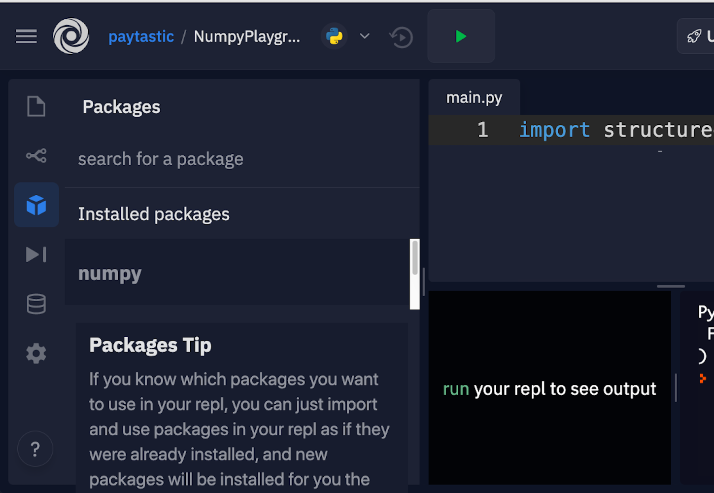
Luckily, they allow you to just click and install.
Installing NumPy With Anaconda
The Anaconda distribution is a suite of common Python data science tools bundled around a package manager that helps manage your virtual environments and project dependencies. It’s built around conda, which is the actual package manager. This is the method recommended by the NumPy project, especially if you’re stepping into data science in Python without having already set up a complex development environment.
If you’ve already got a workflow you like that uses pip, Pipenv, Poetry, or some other toolset, then it might be better not to add conda to the mix. The conda package repository is separate from PyPI, and conda itself sets up a separate little island of packages on your machine, so managing paths and remembering which package lives where can be a nightmare.
Once you’ve got conda installed, you can run the install command for the libraries you’ll need:
$ conda install numpy matplotlib
This will install what you need for this NumPy tutorial, and you’ll be all set to go.
Installing NumPy With pip
Although the NumPy project recommends using conda if you’re starting fresh, there’s nothing wrong with managing your environment yourself and just using good old pip, Pipenv, Poetry, or whatever other alternative to pip is your favorite.
Here are the commands to get set up with pip:
$ mkdir numpy-tutorial
$ cd numpy-tutorial
$ python3 -m venv .numpy-tutorial-venv
$ source .numpy-tutorial-venv/bin/activate
(.numpy-tutorial-venv)
$ pip install numpy matplotlib
Collecting numpy
Downloading numpy-1.19.1-cp38-cp38-macosx_10_9_x86_64.whl (15.3 MB)
|████████████████████████████████| 15.3 MB 2.7 MB/s
Collecting matplotlib
Downloading matplotlib-3.3.0-1-cp38-cp38-macosx_10_9_x86_64.whl (11.4 MB)
|████████████████████████████████| 11.4 MB 16.8 MB/s
...
After this, make sure your virtual environment is activated, and all your code should run as expected.
Using IPython, Notebooks, or JupyterLab
While the above sections should get you everything you need to get started, there are a couple more tools that you can optionally install to make working in data science more developer-friendly.
IPython is an upgraded Python read-eval-print loop (REPL) that makes editing code in a live interpreter session more straightforward and prettier. Here’s what an IPython REPL session looks like:
>>>
In [1]: import numpy as np
In [2]: digits = np.array([
...: [1, 2, 3],
...: [4, 5, 6],
...: [6, 7, 9],
...: ])
In [3]: digits
Out[3]:
array([[1, 2, 3],
[4, 5, 6],
[6, 7, 9]])
It has several differences from a basic Python REPL, including its line numbers, use of colors, and quality of array visualizations. There are also a lot of user-experience bonuses that make it more pleasant to enter, re-enter, and edit code.
You can install IPython as a standalone:
Alternatively, if you wait and install any of the subsequent tools, then they’ll include a copy of IPython.
A slightly more featureful alternative to a REPL is a notebook. Notebooks are a slightly different style of writing Python than standard scripts, though. Instead of a traditional Python file, they give you a series of mini-scripts called cells that you can run and re-run in whatever order you want, all in the same Python memory session.
One neat thing about notebooks is that you can include graphs and render Markdown paragraphs between cells, so they’re really nice for writing up data analyses right inside the code!
Here’s what it looks like:
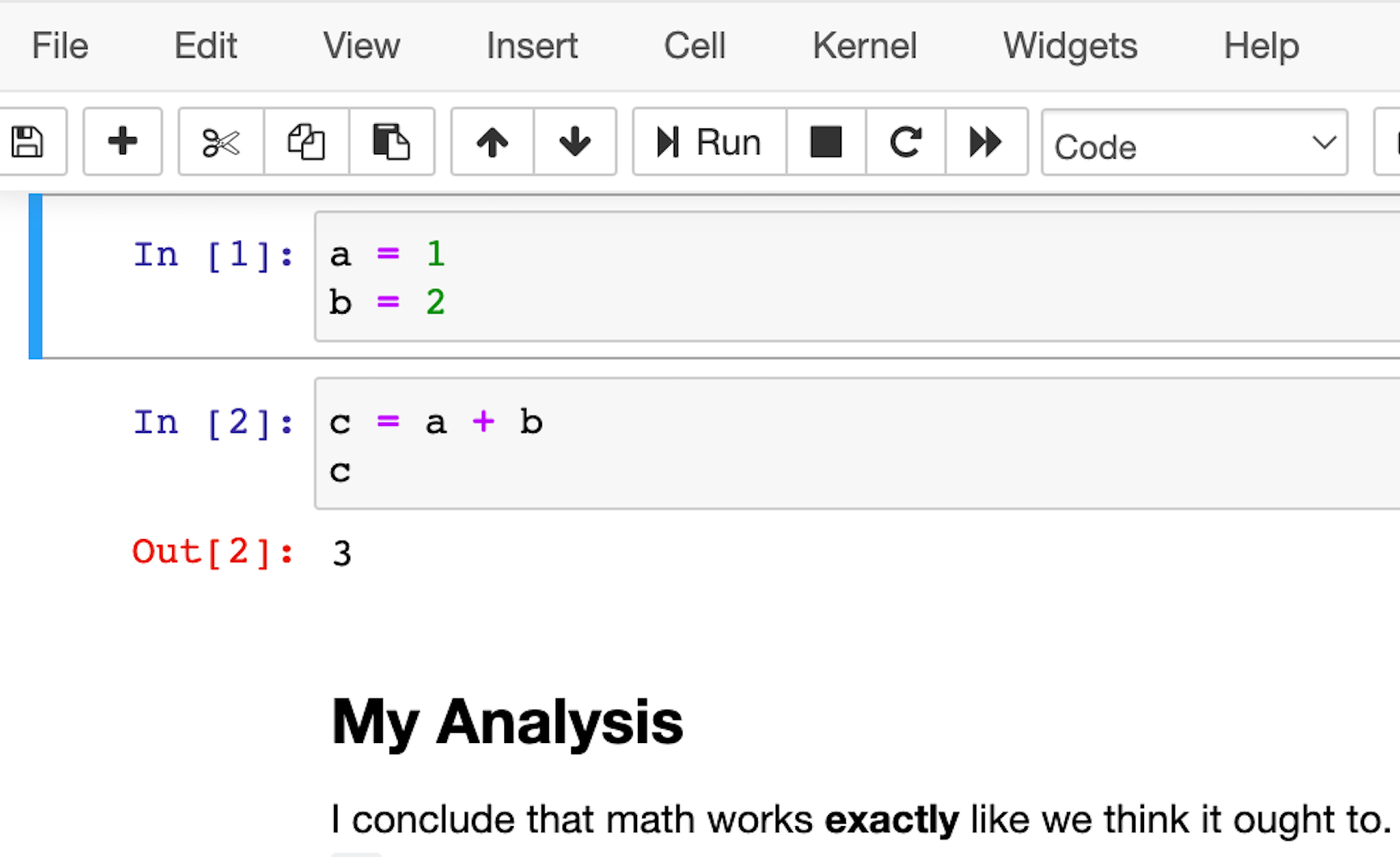
The most popular notebook offering is probably the Jupyter Notebook, but nteract is another option that wraps the Jupyter functionality and attempts to make it a bit more approachable and powerful.
However, if you’re looking at Jupyter Notebook and thinking that it needs more IDE-like qualities, then JupyterLab is another option. You can customize text editors, notebooks, terminals, and custom components, all in a browser-based interface. It will likely be more comfortable for people coming from MatLab. It’s the youngest of the offerings, but its 1.0 release was back in 2019, so it should be stable and full featured.
This is what the interface looks like:
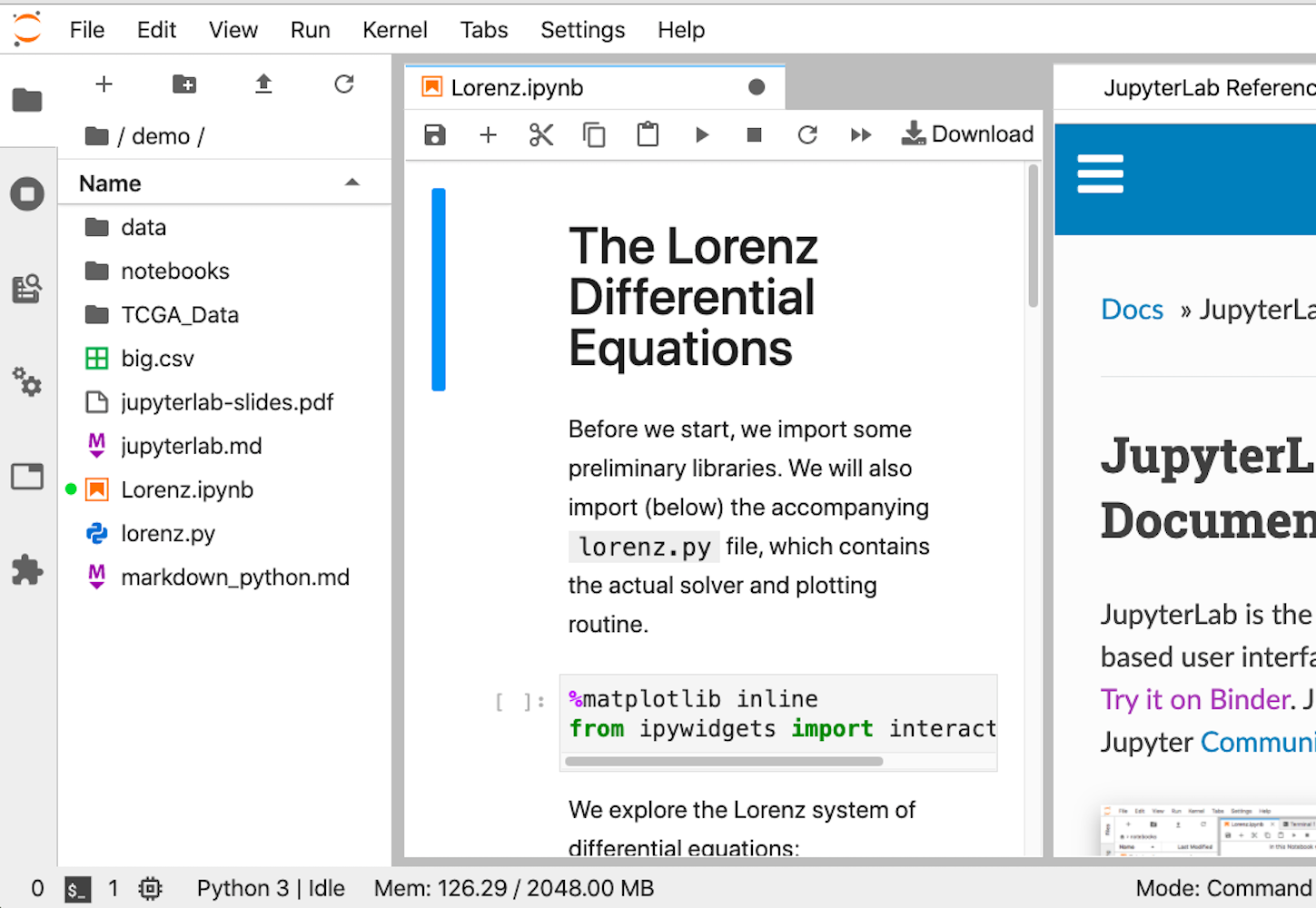
Whichever option you choose, once you have it installed, you’ll be ready to run your first lines of NumPy code. It’s time for the first example.
Hello NumPy: Curving Test Grades Tutorial
This first example introduces a few core concepts in NumPy that you’ll use throughout the rest of the tutorial:
- Creating arrays using
numpy.array() - Treating complete arrays like individual values to make vectorized calculations more readable
- Using built-in NumPy functions to modify and aggregate the data
These concepts are the core of using NumPy effectively.
The scenario is this: You’re a teacher who has just graded your students on a recent test. Unfortunately, you may have made the test too challenging, and most of the students did worse than expected. To help everybody out, you’re going to curve everyone’s grades.
It’ll be a relatively rudimentary curve, though. You’ll take whatever the average score is and declare that a C. Additionally, you’ll make sure that the curve doesn’t accidentally hurt your students’ grades or help so much that the student does better than 100%.
Enter this code into your REPL:
>>>
1>>> import numpy as np
2>>> CURVE_CENTER = 80
3>>> grades = np.array([72, 35, 64, 88, 51, 90, 74, 12])
4>>> def curve(grades):
5... average = grades.mean()
6... change = CURVE_CENTER - average
7... new_grades = grades + change
8... return np.clip(new_grades, grades, 100)
9...
10>>> curve(grades)
11array([ 91.25, 54.25, 83.25, 100. , 70.25, 100. , 93.25, 31.25])
The original scores have been increased based on where they were in the pack, but none of them were pushed over 100%.
Here are the important highlights:
- Line 1 imports NumPy using the
npalias, which is a common convention that saves you a few keystrokes. - Line 3 creates your first NumPy array, which is one-dimensional and has a shape of
(8,)and a data type ofint64. Don’t worry too much about these details yet. You’ll explore them in more detail later in the tutorial. - Line 5 takes the average of all the scores using
.mean(). Arrays have a lot of methods.
On line 7, you take advantage of two important concepts at once:
- Vectorization
- Broadcasting
Vectorization is the process of performing the same operation in the same way for each element in an array. This removes for loops from your code but achieves the same result.
Broadcasting is the process of extending two arrays of different shapes and figuring out how to perform a vectorized calculation between them. Remember, grades is an array of numbers of shape (8,) and change is a scalar, or single number, essentially with shape (1,). In this case, NumPy adds the scalar to each item in the array and returns a new array with the results.
Finally, on line 8, you limit, or clip, the values to a set of minimums and maximums. In addition to array methods, NumPy also has a large number of built-in functions. You don’t need to memorize them all—that’s what documentation is for. Anytime you get stuck or feel like there should be an easier way to do something, take a peek at the documentation and see if there isn’t already a routine that does exactly what you need.
In this case, you need a function that takes an array and makes sure the values don’t exceed a given minimum or maximum. clip() does exactly that.
Line 8 also provides another example of broadcasting. For the second argument to clip(), you pass grades, ensuring that each newly curved grade doesn’t go lower than the original grade. But for the third argument, you pass a single value: 100. NumPy takes that value and broadcasts it against every element in new_grades, ensuring that none of the newly curved grades exceeds a perfect score.
Getting Into Shape: Array Shapes and Axes
Now that you’ve seen some of what NumPy can do, it’s time to firm up that foundation with some important theory. There are a few concepts that are important to keep in mind, especially as you work with arrays in higher dimensions.
Vectors, which are one-dimensional arrays of numbers, are the least complicated to keep track of. Two dimensions aren’t too bad, either, because they’re similar to spreadsheets. But things start to get tricky at three dimensions, and visualizing four? Forget about it.
Mastering Shape
Shape is a key concept when you’re using multidimensional arrays. At a certain point, it’s easier to forget about visualizing the shape of your data and to instead follow some mental rules and trust NumPy to tell you the correct shape.
All arrays have a property called .shape that returns a tuple of the size in each dimension. It’s less important which dimension is which, but it’s critical that the arrays you pass to functions are in the shape that the functions expect. A common way to confirm that your data has the proper shape is to print the data and its shape until you’re sure everything is working like you expect.
This next example will show this process. You’ll create an array with a complex shape, check it, and reorder it to look like it’s supposed to:
>>>
In [1]: import numpy as np
In [2]: temperatures = np.array([
...: 29.3, 42.1, 18.8, 16.1, 38.0, 12.5,
...: 12.6, 49.9, 38.6, 31.3, 9.2, 22.2
...: ]).reshape(2, 2, 3)
In [3]: temperatures.shape
Out[3]: (2, 2, 3)
In [4]: temperatures
Out[4]:
array([[[29.3, 42.1, 18.8],
[16.1, 38. , 12.5]],
[[12.6, 49.9, 38.6],
[31.3, 9.2, 22.2]]])
In [5]: np.swapaxes(temperatures, 1, 2)
Out[5]:
array([[[29.3, 16.1],
[42.1, 38. ],
[18.8, 12.5]],
[[12.6, 31.3],
[49.9, 9.2],
[38.6, 22.2]]])
Here, you use a numpy.ndarray method called .reshape() to form a 2 × 2 × 3 block of data. When you check the shape of your array in input 3, it’s exactly what you told it to be. However, you can see how printed arrays quickly become hard to visualize in three or more dimensions. After you swap axes with .swapaxes(), it becomes little clearer which dimension is which. You’ll see more about axes in the next section.
Shape will come up again in the section on broadcasting. For now, just keep in mind that these little checks don’t cost anything. You can always delete the cells or get rid of the code once things are running smoothly.
Understanding Axes
The example above shows how important it is to know not only what shape your data is in but also which data is in which axis. In NumPy arrays, axes are zero-indexed and identify which dimension is which. For example, a two-dimensional array has a vertical axis (axis 0) and a horizontal axis (axis 1). Lots of functions and commands in NumPy change their behavior based on which axis you tell them to process.
This example will show how .max() behaves by default, with no axis argument, and how it changes functionality depending on which axis you specify when you do supply an argument:
>>>
In [1]: import numpy as np
In [2]: table = np.array([
...: [5, 3, 7, 1],
...: [2, 6, 7 ,9],
...: [1, 1, 1, 1],
...: [4, 3, 2, 0],
...: ])
In [3]: table.max()
Out[3]: 9
In [4]: table.max(axis=0)
Out[4]: array([5, 6, 7, 9])
In [5]: table.max(axis=1)
Out[5]: array([7, 9, 1, 4])
By default, .max() returns the largest value in the entire array, no matter how many dimensions there are. However, once you specify an axis, it performs that calculation for each set of values along that particular axis. For example, with an argument of axis=0, .max() selects the maximum value in each of the four vertical sets of values in table and returns an array that has been flattened, or aggregated into a one-dimensional array.
In fact, many of NumPy’s functions behave this way: If no axis is specified, then they perform an operation on the entire dataset. Otherwise, they perform the operation in an axis-wise fashion.
Broadcasting
So far, you’ve seen a couple of smaller examples of broadcasting, but the topic will start to make more sense the more examples you see. Fundamentally, it functions around one rule: arrays can be broadcast against each other if their dimensions match or if one of the arrays has a size of 1.
If the arrays match in size along an axis, then elements will be operated on element-by-element, similar to how the built-in Python function zip() works. If one of the arrays has a size of 1 in an axis, then that value will be broadcast along that axis, or duplicated as many times as necessary to match the number of elements along that axis in the other array.
Here’s a quick example. Array A has the shape (4, 1, 8), and array B has the shape (1, 6, 8). Based on the rules above, you can operate on these arrays together:
- In axis 0,
Ahas a4andBhas a1, soBcan be broadcast along that axis. - In axis 1,
Ahas a 1 andBhas a 6, soAcan be broadcast along that axis. - In axis 2, the two arrays have matching sizes, so they can operate successfully.
All three axes successfully follow the rule.
You can set up the arrays like this:
>>>
In [1]: import numpy as np
In [2]: A = np.arange(32).reshape(4, 1, 8)
In [3]: A
Out[3]:
array([[[ 0, 1, 2, 3, 4, 5, 6, 7]],
[[ 8, 9, 10, 11, 12, 13, 14, 15]],
[[16, 17, 18, 19, 20, 21, 22, 23]],
[[24, 25, 26, 27, 28, 29, 30, 31]]])
In [4]: B = np.arange(48).reshape(1, 6, 8)
In [5]: B
Out[5]:
array([[[ 0, 1, 2, 3, 4, 5, 6, 7],
[ 8, 9, 10, 11, 12, 13, 14, 15],
[16, 17, 18, 19, 20, 21, 22, 23],
[24, 25, 26, 27, 28, 29, 30, 31],
[32, 33, 34, 35, 36, 37, 38, 39],
[40, 41, 42, 43, 44, 45, 46, 47]]])
A has 4 planes, each with 1 row and 8 columns. B has only 1 plane with 6 rows and 8 columns. Watch what NumPy does for you when you try to do a calculation between them!
Add the two arrays together:
>>>
In [7]: A + B
Out[7]:
array([[[ 0, 2, 4, 6, 8, 10, 12, 14],
[ 8, 10, 12, 14, 16, 18, 20, 22],
[16, 18, 20, 22, 24, 26, 28, 30],
[24, 26, 28, 30, 32, 34, 36, 38],
[32, 34, 36, 38, 40, 42, 44, 46],
[40, 42, 44, 46, 48, 50, 52, 54]],
[[ 8, 10, 12, 14, 16, 18, 20, 22],
[16, 18, 20, 22, 24, 26, 28, 30],
[24, 26, 28, 30, 32, 34, 36, 38],
[32, 34, 36, 38, 40, 42, 44, 46],
[40, 42, 44, 46, 48, 50, 52, 54],
[48, 50, 52, 54, 56, 58, 60, 62]],
[[16, 18, 20, 22, 24, 26, 28, 30],
[24, 26, 28, 30, 32, 34, 36, 38],
[32, 34, 36, 38, 40, 42, 44, 46],
[40, 42, 44, 46, 48, 50, 52, 54],
[48, 50, 52, 54, 56, 58, 60, 62],
[56, 58, 60, 62, 64, 66, 68, 70]],
[[24, 26, 28, 30, 32, 34, 36, 38],
[32, 34, 36, 38, 40, 42, 44, 46],
[40, 42, 44, 46, 48, 50, 52, 54],
[48, 50, 52, 54, 56, 58, 60, 62],
[56, 58, 60, 62, 64, 66, 68, 70],
[64, 66, 68, 70, 72, 74, 76, 78]]])
The way broadcasting works is that NumPy duplicates the plane in B three times so that you have a total of four, matching the number of planes in A. It also duplicates the single row in A five times for a total of six, matching the number of rows in B. Then it adds each element in the newly expanded A array to its counterpart in the same location in B. The result of each calculation shows up in the corresponding location of the output.
Once again, even though you can use words like “plane,” “row,” and “column” to describe how the shapes in this example are broadcast to create matching three-dimensional shapes, things get more complicated at higher dimensions. A lot of times, you’ll have to simply follow the broadcasting rules and do lots of print-outs to make sure things are working as planned.
Understanding broadcasting is an important part of mastering vectorized calculations, and vectorized calculations are the way to write clean, idiomatic NumPy code.
Data Science Operations: Filter, Order, Aggregate
That wraps up a section that was heavy in theory but a little light on practical, real-world examples. In this section, you’ll work through some examples of real, useful data science operations: filtering, sorting, and aggregating data.
Indexing
Indexing uses many of the same idioms that normal Python code uses. You can use positive or negative indices to index from the front or back of the array. You can use a colon (:) to specify “the rest” or “all,” and you can even use two colons to skip elements as with regular Python lists.
Here’s the difference: NumPy arrays use commas between axes, so you can index multiple axes in one set of square brackets. An example is the easiest way to show this off. It’s time to confirm Dürer’s magic square!
The number square below has some amazing properties. If you add up any of the rows, columns, or diagonals, then you’ll get the same number, 34. That’s also what you’ll get if you add up each of the four quadrants, the center four squares, the four corner squares, or the four corner squares of any of the contained 3 × 3 grids. You’re going to prove it!
Enter the following into your REPL:
>>>
In [1]: import numpy as np
In [2]: square = np.array([
...: [16, 3, 2, 13],
...: [5, 10, 11, 8],
...: [9, 6, 7, 12],
...: [4, 15, 14, 1]
...: ])
In [3]: for i in range(4):
...: assert square[:, i].sum() == 34
...: assert square[i, :].sum() == 34
...:
In [4]: assert square[:2, :2].sum() == 34
In [5]: assert square[2:, :2].sum() == 34
In [6]: assert square[:2, 2:].sum() == 34
In [7]: assert square[2:, 2:].sum() == 34
Inside the for loop, you verify that all the rows and all the columns add up to 34. After that, using selective indexing, you verify that each of the quadrants also adds up to 34.
One last thing to note is that you’re able to take the sum of any array to add up all of its elements globally with square.sum(). This method can also take an axis argument to do an axis-wise summing instead.
Masking and Filtering
Index-based selection is great, but what if you want to filter your data based on more complicated nonuniform or nonsequential criteria? This is where the concept of a mask comes into play.
A mask is an array that has the exact same shape as your data, but instead of your values, it holds Boolean values: either True or False. You can use this mask array to index into your data array in nonlinear and complex ways. It will return all of the elements where the Boolean array has a True value.
Here’s an example showing the process, first in slow motion and then how it’s typically done, all in one line:
>>>
In [1]: import numpy as np
In [2]: numbers = np.linspace(5, 50, 24, dtype=int).reshape(4, -1)
In [3]: numbers
Out[3]:
array([[ 5, 6, 8, 10, 12, 14],
[16, 18, 20, 22, 24, 26],
[28, 30, 32, 34, 36, 38],
[40, 42, 44, 46, 48, 50]])
In [4]: mask = numbers % 4 == 0
In [5]: mask
Out[5]:
array([[False, False, True, False, True, False],
[ True, False, True, False, True, False],
[ True, False, True, False, True, False],
[ True, False, True, False, True, False]])
In [6]: numbers[mask]
Out[6]: array([ 8, 12, 16, 20, 24, 28, 32, 36, 40, 44, 48])
In [7]: by_four = numbers[numbers % 4 == 0]
In [8]: by_four
Out[8]: array([ 8, 12, 16, 20, 24, 28, 32, 36, 40, 44, 48])
You’ll see an explanation of the new array creation tricks in input 2 in a moment, but for now, focus on the meat of the example. These are the important parts:
- Input 4 creates the mask by performing a vectorized Boolean computation, taking each element and checking to see if it divides evenly by four. This returns a mask array of the same shape with the element-wise results of the computation.
- Input 6 uses this mask to index into the original
numbersarray. This causes the array to lose its original shape, reducing it to one dimension, but you still get the data you’re looking for. - Input 7 provides a more traditional, idiomatic masked selection that you might see in the wild, with an anonymous filtering array created inline, inside the selection brackets. This syntax is similar to usage in the R programming language.
Coming back to input 2, you encounter three new concepts:
- Using
np.linspace()to generate an evenly spaced array - Setting the
dtypeof an output - Reshaping an array with
-1
np.linspace() generates n numbers evenly distributed between a minimum and a maximum, which is useful for evenly distributed sampling in scientific plotting.
Because of the particular calculation in this example, it makes life easier to have integers in the numbers array. But because the space between 5 and 50 doesn’t divide evenly by 24, the resulting numbers would be floating-point numbers. You specify a dtype of int to force the function to round down and give you whole integers. You’ll see a more detailed discussion of data types later on.
Finally, array.reshape() can take -1 as one of its dimension sizes. That signifies that NumPy should just figure out how big that particular axis needs to be based on the size of the other axes. In this case, with 24 values and a size of 4 in axis 0, axis 1 ends up with a size of 6.
Here’s one more example to show off the power of masked filtering. The normal distribution is a probability distribution in which roughly 95.45% of values occur within two standard deviations of the mean.
You can verify that with a little help from NumPy’s random module for generating random values:
>>>
In [1]: import numpy as np
In [2]: from numpy.random import default_rng
In [3]: rng = default_rng()
In [4]: values = rng.standard_normal(10000)
In [5]: values[:5]
Out[5]: array([ .9779210858, 1.8361585253, -.3641365235,
-.1311344527, 1.286542056 ])
In [6]: std = values.std()
In [7]: std
Out[7]: .9940375551073492
In [8]: filtered = values[(values > -2 * std) & (values < 2 * std)]
In [9]: filtered.size
Out[9]: 9565
In [10]: values.size
Out[10]: 10000
In [11]: filtered.size / values.size
Out[11]: 0.9565
Here you use a potentially strange-looking syntax to combine filter conditions: a binary & operator. Why would that be the case? It’s because NumPy designates & and | as the vectorized, element-wise operators to combine Booleans. If you try to do A and B, then you’ll get a warning about how the truth value for an array is weird, because the and is operating on the truth value of the whole array, not element by element.
Transposing, Sorting, and Concatenating
Other manipulations, while not quite as common as indexing or filtering, can also be very handy depending on the situation you’re in. You’ll see a few examples in this section.
Here’s transposing an array:
>>>
In [1]: import numpy as np
In [2]: a = np.array([
...: [1, 2],
...: [3, 4],
...: [5, 6],
...: ])
In [3]: a.T
Out[3]:
array([[1, 3, 5],
[2, 4, 6]])
In [4]: a.transpose()
Out[4]:
array([[1, 3, 5],
[2, 4, 6]])
When you calculate the transpose of an array, the row and column indices of every element are switched. Item [0, 2], for example, becomes item [2, 0]. You can also use a.T as an alias for a.transpose().
The following code block shows sorting, but you’ll also see a more powerful sorting technique in the coming section on structured data:
>>>
In [1]: import numpy as np
In [2]: data = np.array([
...: [7, 1, 4],
...: [8, 6, 5],
...: [1, 2, 3]
...: ])
In [3]: np.sort(data)
Out[3]:
array([[1, 4, 7],
[5, 6, 8],
[1, 2, 3]])
In [4]: np.sort(data, axis=None)
Out[4]: array([1, 1, 2, 3, 4, 5, 6, 7, 8])
In [5]: np.sort(data, axis=0)
Out[5]:
array([[1, 1, 3],
[7, 2, 4],
[8, 6, 5]])
Omitting the axis argument automatically selects the last and innermost dimension, which is the rows in this example. Using None flattens the array and performs a global sort. Otherwise, you can specify which axis you want. In output 5, each column of the array still has all of its elements but they have been sorted low-to-high inside that column.
Finally, here’s an example of concatenation. While there’s a np.concatenate() function, there are also a number of helper functions that are sometimes easier to read.
Here are some examples:
>>>
In [1]: import numpy as np
In [2]: a = np.array([
...: [4, 8],
...: [6, 1]
...: ])
In [3]: b = np.array([
...: [3, 5],
...: [7, 2],
...: ])
In [4]: np.hstack((a, b))
Out[4]:
array([[4, 8, 3, 5],
[6, 1, 7, 2]])
In [5]: np.vstack((b, a))
Out[5]:
array([[3, 5],
[7, 2],
[4, 8],
[6, 1]])
In [6]: np.concatenate((a, b))
Out[6]:
array([[4, 8],
[6, 1],
[3, 5],
[7, 2]])
In [7]: np.concatenate((a, b), axis=None)
Out[7]: array([4, 8, 6, 1, 3, 5, 7, 2])
Inputs 4 and 5 show the slightly more intuitive functions hstack() and vstack(). Inputs 6 and 7 show the more generic concatenate(), first without an axis argument and then with axis=None. This flattening behavior is similar in form to what you just saw with sort().
One important stumbling block to note is that all these functions take a tuple of arrays as their first argument rather than a variable number of arguments as you might expect. You can tell because there’s an extra pair of parentheses.
Aggregating
Your last stop on this tour of functionality before diving into some more advanced topics and examples is aggregation. You’ve already seen quite a few aggregating methods, including .sum(), .max(), .mean(), and .std(). You can reference NumPy’s larger library of functions to see more. Many of the mathematical, financial, and statistical functions use aggregation to help you reduce the number of dimensions in your data.
Practical Example 1: Implementing a Maclaurin Series
Now it’s time to see a realistic use case for the skills introduced in the sections above: implementing an equation.
One of the hardest things about converting mathematical equations to code without NumPy is that many of the visual similarities are missing, which makes it hard to tell what portion of the equation you’re looking at as you read the code. Summations are converted to more verbose for loops, and limit optimizations end up looking like while loops.
Using NumPy allows you to keep closer to a one-to-one representation from equation to code.
In this next example, you’ll encode the Maclaurin series for ex. Maclaurin series are a way of approximating more complicated functions with an infinite series of summed terms centered about zero.
For ex, the Maclaurin series is the following summation:

You add up terms starting at zero and going theoretically to infinity. Each nth term will be x raised to n and divided by n!, which is the notation for the factorial operation.
Now it’s time for you to put that into NumPy code. Create a file called maclaurin.py:
from math import e, factorial
import numpy as np
fac = np.vectorize(factorial)
def e_x(x, terms=10):
"""Approximates e^x using a given number of terms of
the Maclaurin series
"""
n = np.arange(terms)
return np.sum((x ** n) / fac(n))
if __name__ == "__main__":
print("Actual:", e ** 3) # Using e from the standard library
print("N (terms)tMaclaurintError")
for n in range(1, 14):
maclaurin = e_x(3, terms=n)
print(f"{n}tt{maclaurin:.03f}tt{e**3 - maclaurin:.03f}")
When you run this, you should see the following result:
$ python3 maclaurin.py
Actual: 20.085536923187664
N (terms) Maclaurin Error
1 1.000 19.086
2 4.000 16.086
3 8.500 11.586
4 13.000 7.086
5 16.375 3.711
6 18.400 1.686
7 19.412 0.673
8 19.846 0.239
9 20.009 0.076
10 20.063 0.022
11 20.080 0.006
12 20.084 0.001
13 20.085 0.000
As you increase the number of terms, your Maclaurin value gets closer and closer to the actual value, and your error shrinks smaller and smaller.
The calculation of each term involves taking x to the n power and dividing by n!, or the factorial of n. Adding, summing, and raising to powers are all operations that NumPy can vectorize automatically and quickly, but not so for factorial().
To use factorial() in a vectorized calculation, you have to use np.vectorize() to create a vectorized version. The documentation for np.vectorize() states that it’s little more than a thin wrapper that applies a for loop to a given function. There are no real performance benefits from using it instead of normal Python code, and there are potentially some overhead penalties. However, as you’ll see in a moment, the readability benefits are huge.
Once your vectorized factorial is in place, the actual code to calculate the entire Maclaurin series is shockingly short. It’s also readable. Most importantly, it’s almost exactly one-to-one with how the mathematical equation looks:
n = np.arange(terms)
return np.sum((x ** n) / fac(n))
This is such an important idea that it deserves to be repeated. With the exception of the extra line to initialize n, the code reads almost exactly the same as the original math equation. No for loops, no temporary i, j, k variables. Just plain, clear, math.
Just like that, you’re using NumPy for mathematical programming! For extra practice, try picking one of the other Maclaurin series and implementing it in a similar way.
Optimizing Storage: Data Types
Now that you have a bit more practical experience, it’s time to go back to theory and look at data types. Data types don’t play a central role in a lot of Python code. Numbers work like they’re supposed to, strings do other things, Booleans are true or false, and other than that, you make your own objects and collections.
In NumPy, though, there’s a little more detail that needs to be covered. NumPy uses C code under the hood to optimize performance, and it can’t do that unless all the items in an array are of the same type. That doesn’t just mean the same Python type. They have to be the same underlying C type, with the same shape and size in bits!
Numerical Types: int, bool, float, and complex
Since most of your data science and numerical calculations will tend to involve numbers, they seem like the best place to start. There are essentially four numerical types in NumPy code, and each one can take a few different sizes.
The table below breaks down the details of these types:
| Name | # of Bits | Python Type | NumPy Type |
|---|---|---|---|
| Integer | 64 | int |
np.int_ |
| Booleans | 8 | bool |
np.bool_ |
| Float | 64 | float |
np.float_ |
| Complex | 128 | complex |
np.complex_ |
These are just the types that map to existing Python types. NumPy also has types for the smaller-sized versions of each, like 8-, 16-, and 32-bit integers, 32-bit single-precision floating-point numbers, and 64-bit single-precision complex numbers. The documentation lists them in their entirety.
To specify the type when creating an array, you can provide a dtype argument:
>>>
In [1]: import numpy as np
In [2]: a = np.array([1, 3, 5.5, 7.7, 9.2], dtype=np.single)
In [3]: a
Out[3]: array([1. , 3. , 5.5, 7.7, 9.2], dtype=float32)
In [4]: b = np.array([1, 3, 5.5, 7.7, 9.2], dtype=np.uint8)
In [5]: b
Out[5]: array([1, 3, 5, 7, 9], dtype=uint8)
NumPy automatically converts your platform-independent type np.single to whatever fixed-size type your platform supports for that size. In this case, it uses np.float32. If your provided values don’t match the shape of the dtype you provided, then NumPy will either fix it for you or raise an error.
String Types: Sized Unicode
Strings behave a little strangely in NumPy code because NumPy needs to know how many bytes to expect, which isn’t usually a factor in Python programming. Luckily, NumPy does a pretty good job at taking care of less complex cases for you:
>>>
In [1]: import numpy as np
In [2]: names = np.array(["bob", "amy", "han"], dtype=str)
In [3]: names
Out[3]: array(['bob', 'amy', 'han'], dtype='<U3')
In [4]: names.itemsize
Out[4]: 12
In [5]: names = np.array(["bob", "amy", "han"])
In [6]: names
Out[6]: array(['bob', 'amy', 'han'], dtype='<U3')
In [7]: more_names = np.array(["bobo", "jehosephat"])
In [8]: np.concatenate((names, more_names))
Out[8]: array(['bob', 'amy', 'han', 'bobo', 'jehosephat'], dtype='<U10')
In input 2, you provide a dtype of Python’s built-in str type, but in output 3, it’s been converted into a little-endian Unicode string of size 3. When you check the size of a given item in input 4, you see that they’re each 12 bytes: three 4-byte Unicode characters.
When you combine that with an array that has a larger item to create a new array in input 8, NumPy helpfully figures out how big the new array’s items need to be and grows them all to size <U10.
But here’s what happens when you try to modify one of the slots with a value larger than the capacity of the dtype:
>>>
In [9]: names[2] = "jamima"
In [10]: names
Out[10]: array(['bob', 'amy', 'jam'], dtype='<U3')
It doesn’t work as expected and truncates your value instead. If you already have an array, then NumPy’s automatic size detection won’t work for you. You get three characters and that’s it. The rest get lost in the void.
This is all to say that, in general, NumPy has your back when you’re working with strings, but you should always keep an eye on the size of your elements and make sure you have enough space when modifying or changing arrays in place.
Structured Arrays
Originally, you learned that array items all have to be the same data type, but that wasn’t entirely correct. NumPy has a special kind of array, called a record array or structured array, with which you can specify a type and, optionally, a name on a per-column basis. This makes sorting and filtering even more powerful, and it can feel similar to working with data in Excel, CSVs, or relational databases.
Here’s a quick example to show them off a little:
>>>
In [1]: import numpy as np
In [2]: data = np.array([
...: ("joe", 32, 6),
...: ("mary", 15, 20),
...: ("felipe", 80, 100),
...: ("beyonce", 38, 9001),
...: ], dtype=[("name", str, 10), ("age", int), ("power", int)])
In [3]: data[0]
Out[3]: ('joe', 32, 6)
In [4]: data["name"]
Out[4]: array(['joe', 'mary', 'felipe', 'beyonce'], dtype='<U10')
In [5]: data[data["power"] > 9000]["name"]
Out[5]: array(['beyonce'], dtype='<U10')
In input 2, you create an array, except each item is a tuple with a name, an age, and a power level. For the dtype, you actually provide a list of tuples with the information about each field: name is a 10-character Unicode field, and both age and power are standard 4-byte or 8-byte integers.
In input 3, you can see that the rows, known as records, are still accessible using the index.
In input 4, you see a new syntax for accessing an entire column, or field.
Finally, in input 5, you see a super-powerful combination of mask-based filtering based on a field and field-based selection. Notice how it’s not that much different to read the following SQL query:
SELECT name FROM data
WHERE power > 9000;
In both cases, the result is a list of names where the power level is over 9000.
You can even add in ORDER BY functionality by making use of np.sort():
>>>
In [6]: np.sort(data[data["age"] > 20], order="power")["name"]
Out[6]: array(['joe', 'felipe', 'beyonce'], dtype='<U10')
This sorts the data by power before retrieving it, which rounds out your selection of NumPy tools for selecting, filtering, and sorting items just like you might in SQL!
More on Data Types
This section of the tutorial was designed to get you just enough knowledge to be productive with NumPy’s data types, understand a little of how things work under the hood, and recognize some common pitfalls. It’s certainly not an exhaustive guide. The NumPy documentation on ndarrays has tons more resources.
There’s also a lot more information on dtype objects, including the different ways to construct, customize, and optimize them and how to make them more robust for all your data-handling needs. If you run into trouble and your data isn’t loading into arrays exactly how you expected, then that’s a good place to start.
Lastly, the NumPy recarray is a powerful object in its own right, and you’ve really only scratched the surface of the capabilities of structured datasets. It’s definitely worth reading through the recarray documentation as well as the documentation for the other specialized array subclasses that NumPy provides.
Looking Ahead: More Powerful Libraries
In this next section, you’ll move on to the powerhouse tools that are built on top of the foundational building blocks you saw above. Here are a few of the libraries that you’ll want to take a look at as your next steps on the road to total Python data science mastery.
pandas
pandas is a library that takes the concept of structured arrays and builds it out with tons of convenience methods, developer-experience improvements, and better automation. If you need to import data from basically anywhere, clean it, reshape it, polish it, and then export it into basically any format, then pandas is the library for you. It’s likely that at some point, you’ll import pandas as pd at the same time you import numpy as np.
The pandas documentation has a speedy tutorial filled with concrete examples called 10 Minutes to pandas. It’s a great resource that you can use to get some quick, hands-on practice.
scikit-learn
If your goals lie more in the direction of machine learning, then scikit-learn is the next step. Given enough data, you can do classification, regression, clustering, and more in just a few lines.
If you’re already comfortable with the math, then the scikit-learn documentation has a great list of tutorials to get you up and running in Python. If not, then the Math for Data Science Learning Path is a good place to start. Additionally, there’s also an entire learning path for machine learning.
It’s important for you to understand at least the basics of the mathematics behind the algorithms rather than just importing them and running with it. Bias in machine learning models is a huge ethical, social, and political issue.
Throwing data at models without a considering how to address the bias is a great way to get into trouble and negatively impact people’s lives. Doing some research and learning how to predict where bias might occur is a good start in the right direction.
Matplotlib
No matter what you’re doing with your data, at some point you’ll need to communicate your results to other humans, and Matplotlib is one of the main libraries for making that happen. For an introduction, check out Plotting with Matplotlib. In the next section, you’ll get some hands-on practice with Matplotlib, but you’ll use it for image manipulation rather than for making plots.
Practical Example 2: Manipulating Images With Matplotlib
It’s always neat when you’re working with a Python library and it hands you something that turns out to be a basic NumPy array. In this example, you’ll experience that in all its glory.
You’re going to load an image using Matplotlib, realize that RGB images are really just width × height × 3 arrays of int8 integers, manipulate those bytes, and use Matplotlib again to save that modified image once you’re done.
Download this image to work with:

It’s a picture of an adorable kitten that is 1920 pixels by 1299 pixels. You’re going to change the colors of those pixels.
Create a Python file called image_mod.py, then set up your imports and load the image:
1import numpy as np
2import matplotlib.image as mpimg
3
4img = mpimg.imread("kitty.jpg")
5print(type(img))
6print(img.shape)
This is a good start. Matplotlib has its own module for handling images, and you’re going to lean on that because it makes straightforward to read and write image formats.
If you run this code, then your friend the NumPy array will appear in the output:
$ python3 image_mod.py
<class 'numpy.ndarray'>
(1299, 1920, 3)
It’s an image with a height of 1299 pixels, a width of 1920 pixels, and three channels: one each for the red, green, and blue (RGB) color levels.
Want to see what happens when you drop out the R and G channels? Add this to your script:
7output = img.copy() # The original image is read-only!
8output[:, :, :2] = 0
9mpimg.imsave("blue.jpg", output)
Run it again and check the folder. There should be a new image:

Is your mind blown yet? Do you feel the power? Images are just fancy arrays! Pixels are just numbers!
But now, it’s time to do something a little more useful. You’re going to convert this image to grayscale. However, converting to grayscale is more complicated. Averaging the R, G, and B channels and making them all the same will give you an image that’s grayscale. But the human brain is weird, and that conversion doesn’t seem to handle the luminosity of the colors quite right.
In fact, it’s better to see it for yourself. You can use the fact that if you output an array with only one channel instead of three, then you can specify a color map, known as a cmap in the Matplotlib world. If you specify a cmap, then Matplotlib will handle the linear gradient calculations for you.
Get rid of the last three lines in your script and replace them with this:
7averages = img.mean(axis=2) # Take the average of each R, G, and B
8mpimg.imsave("bad-gray.jpg", averages, cmap="gray")
These new lines create a new array called averages, which is a copy of the img array that you’ve flattened along axis 2 by taking the average of all three channels. You’ve averaged all three channels and outputted something with R, G, and B values equal to that average. When R, G, and B are all the same, the resulting color is on the grayscale.
What it ends up yielding isn’t terrible:

But you can do better using the luminosity method. This technique does a weighted average of the three channels, with the mindset that the color green drives how bright an image appears to be, and blue can make it appear darker. You’ll use the @ operator, which is NumPy’s operator for doing a traditional two-dimensional array dot product.
Replace those last two lines in your script again:
7weights = np.array([0.3, 0.59, 0.11])
8grayscale = img @ weights
9mpimg.imsave("good-gray.jpg", grayscale, cmap="gray")
This time, instead of doing a flat average, you’re completing a dot product, which is a sort of weighted combination of the three values. Since the weights add up to one, it’s exactly equivalent to doing a weighted average of the three color channels.
Here’s the result:

The first image is a bit darker, and the edges and shadows are bolder. The second image is lighter and brighter, and the dark lines aren’t quite as bold. There you have it—you used Matplotlib and NumPy arrays to manipulate an image!
Conclusion
No matter how many dimensions your data lives in, NumPy gives you the tools to work with it. You can store it, reshape it, combine it, filter it, and sort it, and your code will read like you’re operating on only one number at a time rather than hundreds or thousands.
In this tutorial, you learned:
- The core concepts of data science made possible by NumPy
- How to create NumPy arrays using various methods
- How to manipulate NumPy arrays to perform useful calculations
- How to apply these new skills to real-world problems
Don’t forget to check out the repository of NumPy code samples from throughout this tutorial. You can use it for reference and experiment with the examples to see how changing the code changes the outcome:
Now you’re ready for the next steps in your data science journey. Whether you’re cleaning data, training neural networks, communicating using powerful plots, or aggregating data from the Internet of Things, these activities all start from the same place: the humble NumPy array.
Data Science Tutorial
PySpark Machine Learning Tutorial for Beginners
Snowflake Data Warehouse Tutorial for Beginners with Examples
Jupyter Notebook Tutorial — A Complete Beginners Guide
Best Python NumPy Tutorial for Beginners
Tableau Tutorial for Beginners -Step by Step Guide
MLOps Python Tutorial for Beginners -Get Started with MLOps
Alteryx Tutorial for Beginners to Master Alteryx in 2021
Free Microsoft Power BI Tutorial for Beginners with Examples
Theano Deep Learning Tutorial for Beginners
Computer Vision Tutorial for Beginners | Learn Computer Vision
Python Pandas Tutorial for Beginners — The A-Z Guide
NumPy Python Tutorial for Beginners
Hadoop Online Tutorial – Hadoop HDFS Commands Guide
MapReduce Tutorial–Learn to implement Hadoop WordCount Example
Hadoop Hive Tutorial-Usage of Hive Commands in HQL
Hive Tutorial-Getting Started with Hive Installation on Ubuntu
Learn Java for Hadoop Tutorial: Inheritance and Interfaces
Learn Java for Hadoop Tutorial: Classes and Objects
Learn Java for Hadoop Tutorial: Arrays
Apache Spark Tutorial — Run your First Spark Program
Best PySpark Tutorial for Beginners-Learn Spark with Python
R Tutorial- Learn Data Visualization with R using GGVIS
Neural Network Training Tutorial
Python List Tutorial
MatPlotLib Tutorial
Decision Tree Tutorial
Neural Network Tutorial
Performance Metrics for Machine Learning Algorithms
R Tutorial: Data.Table
SciPy Tutorial
Step-by-Step Apache Spark Installation Tutorial
Introduction to Apache Spark Tutorial
R Tutorial: Importing Data from Web
R Tutorial: Importing Data from Relational Database
R Tutorial: Importing Data from Excel
Introduction to Machine Learning Tutorial
Machine Learning Tutorial: Linear Regression
Machine Learning Tutorial: Logistic Regression
Support Vector Machine Tutorial (SVM)
K-Means Clustering Tutorial
dplyr Manipulation Verbs
Introduction to dplyr package
Importing Data from Flat Files in R
Principal Component Analysis Tutorial
Pandas Tutorial Part-3
Pandas Tutorial Part-2
Pandas Tutorial Part-1
Tutorial- Hadoop Multinode Cluster Setup on Ubuntu
Data Visualizations Tools in R
R Statistical and Language tutorial
Introduction to Data Science with R
Apache Pig Tutorial: User Defined Function Example
Apache Pig Tutorial Example: Web Log Server Analytics
Impala Case Study: Web Traffic
Impala Case Study: Flight Data Analysis
Hadoop Impala Tutorial
Apache Hive Tutorial: Tables
Flume Hadoop Tutorial: Twitter Data Extraction
Flume Hadoop Tutorial: Website Log Aggregation
Hadoop Sqoop Tutorial: Example Data Export
Hadoop Sqoop Tutorial: Example of Data Aggregation
Apache Zookepeer Tutorial: Example of Watch Notification
Apache Zookepeer Tutorial: Centralized Configuration Management
Hadoop Zookeeper Tutorial for Beginners
Hadoop Sqoop Tutorial
Hadoop PIG Tutorial
Hadoop Oozie Tutorial
Hadoop NoSQL Database Tutorial
Hadoop Hive Tutorial
Hadoop HDFS Tutorial
Hadoop hBase Tutorial
Hadoop Flume Tutorial
Hadoop 2.0 YARN Tutorial
Hadoop MapReduce Tutorial
Big Data Hadoop Tutorial for Beginners- Hadoop Installation