![]()
![]()
![]()
![]()
Блог
-
Вы здесь:
- О компании
- Блог
- Десять основных шагов расчета динамических задач в явной постановке. Часть вторая.

В предыдущей статье я изложил первые шесть шагов, необходимых для создания надежных, быстрых и точных моделей для динамических расчётов в явной постановке (Explicit Dynamics). В этой статье я представлю следующие четыре шага. Хочу обратить ваше внимание на то, что описанные шаги являются довольно общими и применимы практически ко всем динамическим расчётам в явной постановке. Однако в особых случаях, возможно, будут необходимы дополнительные настройки. Например, для расчёта взрывного процесса может быть задана расчётная область в постановке Эйлера для моделирования непосредственно взрыва, а затем включены специальные механизмы связанных расчётов для моделирования взаимодействия детонационных газов и твердых тел.
 и явной (справа) постановках")
Пошаговое изложение ключевых аспектов создания моделей для расчёта динамических задач в явной постановке (модули Explicit Dynamics):
7. Создайте сетку.
- Создайте сетку с относительно равномерным распределением размеров элементов. Зоны модели с очень мелкой сеткой приведут к увеличению времени расчета за счет уменьшения потребного шага по времени. На рисунке 1, приведенном выше, показано сравнение предпочтительных сеток для моделей в явной (explicit) и неявной (implicit) постановках расчёта. В динамическом расчёте высокоэнергетических процессов за счёт перемещения и взаимодействия волн колебаний максимальные напряжения могут возникать практически в любом месте, так что для расчёта в явной постановке наличие мелкой сетки в местах скруглений не представляет большой важности.
Некоторые инструменты создания сетки в ANSYS Workbench/LS-Dyna, такие как виртуальная топология (virtual topology) и построение сетки с упрощением геометрии (defeaturing), предоставляют возможности для создания сетки без жесткой привязки к геометрическим элементам. Это значит, что сетка не должна совпадать с границами геометрических поверхностей. Ниже на рисунке 2 показан пример, где созданная по умолчанию сетка содержит очень мелкие элементы на узких поверхностях, присутствующих в показанной слева геометрической модели. Относительно равномерная сетка (нижний рисунок справа) значительно предпочтительнее, поскольку она позволяет существенно сократить время расчета за счет увеличения шага по времени. и более предпочтительная сетка, созданная с помощью виртуальной топологии (справа внизу) – обе созданы на одной и той же геометрии, содержащей узкие грани")
- Используйте как можно больше гексагональных элементов. Элементы в форме тетраэдров не только существенно увеличивают размер модели, но и, как правило, значительно уменьшают потребный шаг по времени.
 и более предпочтительная сетка, созданная с помощью виртуальной топологии (справа внизу) – обе созданы на одной и той же геометрии, содержащей узкие грани")
8. Задайте начальные условия, нагрузки и граничные условия.
- Задайте начальные условия, такие как начальные скорости поступательного и вращательного движения.
- Используйте гладкие кривые изменения нагрузки (например, синусоидальный закон) – это помогает сгладить ударные эффекты.
- Перед запуском решения выведите список и/или выведите графики изменения нагрузок для проверки.
- Для квазистатических расчётов используйте большую скорость и редуцированный расчёт (reduced transient analysis), чтобы уменьшить время расчета. Более подробную информацию о квазистатическом расчёте вы можете найти в моей статье под названием «Чем может помочь решатель для задач в явной постановке в сложных нелинейных статических расчётах?» (How Can Explicit Solvers Help With Stubborn Nonlinear Statics Models?)
9. Создайте и отобразите контактные взаимодействия.
- a) Для оболочечных моделей предпочтительнее выбирать те типы контактов, которые позволяют определять статус контакта на обеих сторонах оболочки. К ним относятся автоматические типы контактов в LS-Dyna.
- b) Не забудьте включить в контактные пары все поверхности, по которым может возникнуть контакт.
- c) При необходимости используйте тип контакта, который поддерживает контактное взаимодействие при самокасании поверхности. Это может понадобиться при смятии конструкции, что часто возникает при расчёте удара автомобиля или моделировании технологических процессов обработки металлов давлением. На рисунке 3 показан пример такого деформирования – сжатие швеллера.
- d) По возможности избегайте начального проникновения. Оно может создавать ложные напряжения, погрешности в определении энергии, а также приводить к нежелательным искажениям геометрии оболочки.


10. Задайте настройки решателя и запустите расчет.
- Укажите время переходного процесса.
- Укажите периодичность вывода результатов. Необходимо использовать достаточное количество точек для того, чтобы были зафиксированы результаты в важные моменты времени, но излишне большое количество точек может привести к переизбытку данных.
По возможности получайте данные с мелким шагом по времени только для совокупности узлов и элементов в важных и интересующих вас зонах. - Запросите вывод таких результатов, как энергия в модели в целом и в каждой детали, силы реакции и силы контактного взаимодействия. Вывод результатов по энергиям является критически важным с точки зрения проверки ошибок. Например, если энергия, соответствующая нефизичному характеру деформирования типа «песочные часы» (hourglass energy), очень высока, то есть на это деформирование уходит существенная доля общей энергии, это говорит о том, что необходимо уделить особое внимание специальным моделям для устранения этого эффекта. Кроме того, сумма первоначальной энергии и работы внешних сил всегда должна быть примерно равна полной энергии системы в любой момент времени.
- Разумно используйте массовое масштабирование (mass scaling). Массовое масштабирование – это надежный и проверенный метод для сокращения времени квазистатических расчётов, где скорость процесса мала, а кинетическая энергия пренебрежима в сравнении с энергией деформирования. При грамотном применении в определенных случаях его также можно применять для динамических расчетов. Больше информации о массовом масштабировании вы можете найти в моей статье под названием «Что такое массовое масштабирование, и когда его уместно применять для динамических расчётов в явной постановке?» (What is Mass Scaling and When is it Appropriate in Explicit Dynamics Analysis?)
Теперь у вас есть полный список шагов, необходимых для создания надежных, быстрых и точных моделей для динамических расчётов в явной постановке (Explicit Dynamics). Я попытался представить дополнительные подробности для шагов, которые специфичны для расчётов явной динамики. Надеюсь, это описание поможет для первоначального знакомства или для развития ваших навыков в этом типе расчётов.
Источник: https://caeai.com/blog/top-ten-list-explicit-dynamics-analysis-part-2
Автор: Steven Hale
Продукты
Услуги
Новости
Блог
What is the Explicit Method?
In the last 15 years, Ansys has gone from offering a single explicit dynamics workflow, using Mechanical APDL with a third-party solver and postprocessor, to offering several unique and versatile solutions. These days Ansys customers can leverage two distinct solvers and multiple pre and post processors in various combinations in order to best meet their needs. However, before a user can determine the right explicit solution for themselves, they must first understand what the term “explicit dynamics” means and what sort of problems that methodology is meant to tackle.
Implicit vs. Explicit Methods in FEA
Traditionally, finite element analysis of a transient structural system is carried out using an implicit solutions method; this approach involves two key principles:
- The assembly of the mass, stiffness, and damping matrices to describe the inherent factors relating to the motion of the structure.
- The approximated solution an ordinary differential equation describing that motion:
 For those inclined to stare blankly at the first sign of math, this equation of motion essentially shows that any external force acting on an object will result in displacement (u vector), velocity (v vector) and acceleration (a vector) of that object. The magnitude of that motion will be inversely related to the stiffness in the system (K matrix), the amount of damping (C matrix), and the mass of the system (M matrix). You can think of these matrices as how springy or elastic the material in use is, how much kinetic energy loss occurs due to heat or sound, and how much resistance to a change in velocity exists respectively. Things get further complicated by the fact that displacement, velocity, and acceleration are all interrelated in a way that makes these equations very difficult to solve directly.
The other significant concept here is the use of matrices to define behavior of a complex system. Since FEA in general involves a component or assembly of components that are broken down into many nodes with many more connections to adjacent nodes, the equations of motion for each node starts to get complicated very quickly. Matrices are a way to describe these complex systems in an organized way that allows a solver to take advantage of certain operations possible in linear algebra.
Consider this 1-dimensional system of springs and nodes. Note that we are only considering the elastic (displacement-related) portion of the motion equations and not inertial (acceleration) or damping (velocity):
The total force acting on, and displacement of each node is going to be related to the relative displacement of the adjacent node or nodes and the stiffness of the springs connecting them. Using a stiffness matrix, we can describe the behavior of the entire system mathematically:
This might look somewhat familiar if you look at the first part of that motion-equation we looked at earlier. In this case, we’re looking at the global stiffness matrix of a simple system as opposed to the matrix of a single node or object. The stiffness between nodes in a finite element model can be thought of as being very similar to the springs’ stiffness in our simple system, and the mass of the system and damping properties can be thought of very similarly to the stiffness in terms of matrix assembly.
So, where are we going with all this? Well, FEA software uses a linear algebraic approach to simplify these matrices before attempting to solve the full equations of motion of the system. In fact, much of the CPU time consumed during the solve process is taken up by this matrix “decomposition” as it is known. Additionally, because the full transient equations of motion can’t easily be solved directly from one point in time to the next, a set of values known as Newmark’s Parameters are used to approximate an incremental change of displacement, velocity, and acceleration between time-steps. The most common method of leveraging these parameters is known as the Newton-Raphson iteration, and involves an iterative approach to solving for the force on any node in the system.
It works like this: the starting position, velocity, and acceleration of the system are known, so the matrices at this state act as our starting point. For the first time increment, a set of matrices modified using the Newmark’s Parameters are formulated and a test force is applied at each node. This test force will result in a new set of positions, velocities, and accelerations at each nodal location. This newly calculated equilibrium state will also result in a new set of calculated forces at each node, and this calculated force can then be compared to the test force. Usually the first iteration will not result in values that fall within a range resulting in an acceptable residual value, so the matrices will be further modified from this first attempt and the process will repeat. This same process repeats until the test force and the calculated force are close enough to be considered converged.
That, in a nutshell, is how the implicit transient method works. In contrast, explicit dynamics takes a different approach to solving motion equations altogether. Instead of using a test force value and incrementally adjusting the system matrices until that test force value matches the resultant equilibrium forces, the explicit approach involves simply integrating the acceleration and velocity terms in the equations over a short period. This results in equations that are defined in terms of displacement alone, meaning they can be solved without the need for convergence toward a solution! Not only that, but this approach also bypasses the need for matrix assembly and decomposition as well, meaning no need for the solver to spend all that time building and simplifying a matrix.
By getting rid of these two often onerous steps, the explicit method allows users to tackle highly complex and nonlinear problems that would otherwise be very difficult to converge (and in many cases it can do so much, much faster). In fact, the Explicit method can be used for some very sophisticated analyses, such as simulating breakage (elements being deleted from the simulation) based on a limit strain value, because the solution at a timestep does not need to converge based on the state of the system at a previous step.
You might be thinking, “Great! Clearly the explicit method is superior. Why wouldn’t we use that approach for everything?” Well, here is the rub: explicit study requires that the analysis be both time-dependent (or transient), and that a minimum time step size be used. The explicit dynamic EOMs are probably not worth showing in their entirety, but one particular term is the issue here:
That innocuous-looking little term might look familiar if you know the equation for the natural frequency of an oscillator:
The significance here is that if the timestep of the explicit analysis, identified here as Δt_i, is longer than the shortest period corresponding to the natural frequencies of the system divided by pi, the motion equation becomes unstable and can’t be solved.
The natural frequencies of the system are sensitive to numerous factors, most significant here are that this period for the natural frequency will decrease with:
- Increasing material stiffness
- Decreasing material density or decreasing mass
- Decreasing size of the SMALLEST element in the entire model
Therefore, the stiffer, more massive, and smaller that smallest element in the model is, the shorter our timestep needs to be to get a solution. And these timesteps can be a tiny fraction of a millionth of a second in many cases! Therefore, even though the Explicit method is a more direct way of solving the equations involved, depending on the problem involved, it might still be more efficient to approach with an implicit solver because of the numerous timesteps necessary for an explicit solution.
Here’s the Bottom Line
The Implicit approach is still a robust and reliable method for solving FEA problems, and usually is the more time and effort-friendly approach for static cases or those that don’t involve much nonlinearity. However, whenever a simulation involves very rapid changes to the state of the model, involves large amounts of deformation or material nonlinearity, or deletion of elements based on material failure, the explicit method excels.
High/Hyper-Velocity Impact and Material FailureFoam and other Highly Non-linear Material
Blast/Explosion/Deflagration
Explicit dynamics can also be very useful for simulating snap-through behavior, metal forming operations, and any number of other events that might otherwise be impossible with the implicit approach. In part 2, we will explore the Ansys Explicit Dynamics portfolio and discuss how each software stacks up against the others in some key areas.
The comments to this entry are closed.
It happens to everyone. You reach to answer your phone, grab it wrong, and suddenly it’s falling — kerplunk! — onto the hard floor. For engineers, knowing how their products will stand up in scenarios like free falls is critical to achieving their safety and performance goals. To test their designs in these highly nonlinear, high-speed situations, they rely on a simulation methodology called explicit dynamics analysis.
Explicit dynamics is a time integration method used to perform dynamic simulations when speed is important. Explicit dynamics account for quickly changing conditions or discontinuous events, such as free falls, high-speed impacts, and applied loads. Because these “nonlinear dynamics” are integrated into the simulation, explicit dynamics is the preferred choice for simulating highly transient physical phenomena.

Explicit Dynamics Capabilities
Explicit dynamics tools help engineers to explore a wide range of challenges:
- Short-duration, complex or changing-body interactions (contact)
- Quasi-static loads (low strain rates)
- High-speed and hypervelocity impacts
- Severe loadings resulting in large material deformation
- Material failure
- Material fragmentation
- Penetration mechanics
- Space debris impact (hypervelocity)
- Sports equipment design
- Manufacturing processes with nonlinear plastic response
- Drop-test simulation
- Explosive loading
- Explosive forming
- Blast-structure interactions
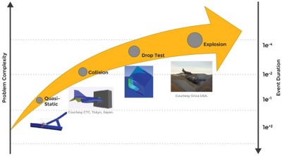
Figure 1. Ansys explicit dynamics tools help users meet solution requirements of various complexities based on problem details and user expertise.
If your product needs to survive impacts or short-duration, high-pressure loadings, you can improve its design with Ansys explicit dynamics solutions. Specialized problems require advanced analysis tools to accurately predict the effect of design considerations on product or process behavior. Gaining insight into such a complex reality is especially important when it is too expensive — or impossible — to perform physical testing.
The Ansys explicit dynamics suite enables you to capture the physics of short-duration events for products that undergo highly nonlinear, transient dynamic forces. Our specialized, accurate, and easy-to-use explicit dynamics tools have been designed to maximize user productivity.
With Ansys, engineers can gain insight into how a structure responds when subjected to severe loadings. Algorithms based on first principles accurately predict complex responses, such as large material deformations and failure, interactions between bodies, and fluids with rapidly deforming structures. Highly complex problems, especially ones with high strain rates and other phenomena that are difficult to converge with general-purpose implicit solution methods, can be resolved using sophisticated, state-of-the-art mathematical algorithms.
Defaults are safe and reasonable for most common problems, which means that you spend less time setting up and running problems and more time optimizing products for performance, durability, and cost, and removing design flaws.
In many cases, the accuracy of an explicit solution can be verified only through comparison with physical experiments. For some problems (such as explosions), it may be too expensive or even impossible to perform physical tests. Despite this, Ansys users around the world rely on the precision of our explicit simulation results.
While both implicit and explicit methods are used to solve time-dependent simulations, deciding which one to use depends on the problem being solved.
Use implicit dynamics when solving for dynamic finite element analysis (FEA) problems that involve mild nonlinearity and when large timesteps can be used. This includes:
- Static equilibriums.
- Slow, linear, and mildly nonlinear processes.
- Large time increments.
Use explicit dynamics when calculating highly complex and nonlinear problems involving rapid changes such as deformation or failure of material, such as:
- Drop tests.
- Impact and penetration.
- Breakage.
- Shock waves.
- Large deformations.
Ansys LS-DYNA
Ansys LS-DYNA is the most frequently used explicit simulation program in the world, capable of simulating applications like drop tests, impact and penetration, smashes and crashes, occupant safety, and more.
Ansys Explict Dynamics within Ansys Mechanical
Ansys Mechanical is the best-in-class finite element solver offering structural, thermal, acoustics, transient, and nonlinear capabilities to solve your most complex structural engineering problems.
Ansys Autodyn
Ansys Autodyn offers a range of models to represent complex physical phenomena such as the interaction of liquids, solids and gases; the phase transitions of materials; the propagation of shock waves; and even explosions.
For solving highly transient, highly nonlinear simulations, explicit dynamics is the preferred choice of time integration methods. To learn about the industry’s leading explicit simulation software, check out the Ansys LS-DYNA Multiphysics Solver.
В шеллах именно по WB DesignModeller — как я понимаю сделать солид, потом на него наложить mid-surface?
Или именно тип тела должен быть surface?
Тип — Surface. Не столько должен, сколько это разумно.
Справитесь ли Вы, просто используя функцию mid-surface, зависит от Вас и от геометрии. Скорее всего, придется поработать над геометрией чуть больше.
В целом, геометрия будет представлена оболочкой и объемными телами, а также, возможно, присоединенными массами.
Верна ли логика — максимально возможный размер элемента?
Шаг по времени, которым Вы недовольны, определяется самым маленьким элементом. Когда таких маленьких элементов несколько штук — может выручить Mass Scaling. В общем и целом лучше обходиться без них.
Логика — избегать ненужного локального измельчения сетки.
Начните с задачки попроще, замените свой грузовик на ящик из shell’ов. Обратите внимание как сетка влияет на шаг по времени(метод сетки Uniform Quad оптимальный). Потом усложняйте геометрию. Потом прицепите пару solid’ов в модель. Убедитесь, что контакты настроены правильно и ничего не разваливается.
Пока с такой задачкой справитесь, освоите практически все, что нужно для Вашего краш-теста.
ANSYS Explicit Dynamics Analysis Guide
ANSYS, Inc. Southpointe 2600 ANSYS Drive Canonsburg, PA 15317 [email protected] http://www.ansys.com (T) 724-746-3304 (F) 724-514-9494
Release 17.0 January 2016 ANSYS, Inc. is certified to ISO 9001:2008.
Copyright and Trademark Information © 2015 SAS IP, Inc. All rights reserved. Unauthorized use, distribution or duplication is prohibited. ANSYS, ANSYS Workbench, Ansoft, AUTODYN, EKM, Engineering Knowledge Manager, CFX, FLUENT, HFSS, AIM and any and all ANSYS, Inc. brand, product, service and feature names, logos and slogans are registered trademarks or trademarks of ANSYS, Inc. or its subsidiaries in the United States or other countries. ICEM CFD is a trademark used by ANSYS, Inc. under license. CFX is a trademark of Sony Corporation in Japan. All other brand, product, service and feature names or trademarks are the property of their respective owners.
Disclaimer Notice THIS ANSYS SOFTWARE PRODUCT AND PROGRAM DOCUMENTATION INCLUDE TRADE SECRETS AND ARE CONFIDENTIAL AND PROPRIETARY PRODUCTS OF ANSYS, INC., ITS SUBSIDIARIES, OR LICENSORS. The software products and documentation are furnished by ANSYS, Inc., its subsidiaries, or affiliates under a software license agreement that contains provisions concerning non-disclosure, copying, length and nature of use, compliance with exporting laws, warranties, disclaimers, limitations of liability, and remedies, and other provisions. The software products and documentation may be used, disclosed, transferred, or copied only in accordance with the terms and conditions of that software license agreement. ANSYS, Inc. is certified to ISO 9001:2008.
U.S. Government Rights For U.S. Government users, except as specifically granted by the ANSYS, Inc. software license agreement, the use, duplication, or disclosure by the United States Government is subject to restrictions stated in the ANSYS, Inc. software license agreement and FAR 12.212 (for non-DOD licenses).
Third-Party Software See the legal information in the product help files for the complete Legal Notice for ANSYS proprietary software and third-party software. If you are unable to access the Legal Notice, Contact ANSYS, Inc. Published in the U.S.A.
Table of Contents 1. Explicit Dynamics Analysis Guide Overview ………………………………………………………………………………. 1 2. Explicit Dynamics Workflow ……………………………………………………………………………………………………. 3 2.1. Introduction ……………………………………………………………………………………………………………………. 3 2.2. Create the Analysis System …………………………………………………………………………………………………. 4 2.3. Define Engineering Data ……………………………………………………………………………………………………. 4 2.4. Attach Geometry ……………………………………………………………………………………………………………… 4 2.5. Define Part Behavior …………………………………………………………………………………………………………. 6 2.6. Define Connections ………………………………………………………………………………………………………….. 7 2.6.1. Spot Welds in Explicit Dynamics Analyses ……………………………………………………………………… 8 2.6.2. Body Interactions in Explicit Dynamics Analyses …………………………………………………………….. 9 2.6.2.1. Properties for Body Interactions Folder ………………………………………………………………… 11 2.6.2.1.1. Contact Detection ……………………………………………………………………………………. 11 2.6.2.1.2. Formulation ……………………………………………………………………………………………. 13 2.6.2.1.3. Shell Thickness Factor and Nodal Shell Thickness …………………………………………… 14 2.6.2.1.4. Body Self Contact …………………………………………………………………………………….. 14 2.6.2.1.5. Element Self Contact ………………………………………………………………………………… 14 2.6.2.1.6. Tolerance ……………………………………………………………………………………………….. 15 2.6.2.1.7. Pinball Factor ………………………………………………………………………………………….. 15 2.6.2.1.8. Time Step Safety Factor …………………………………………………………………………….. 16 2.6.2.1.9. Limiting Time Step Velocity ……………………………………………………………………….. 16 2.6.2.1.10. Edge on Edge Contact …………………………………………………………………………….. 16 2.6.2.2. Interaction Type Properties for Body Interaction Object ………………………………………….. 16 2.6.2.2.1. Frictionless Type ……………………………………………………………………………………… 16 2.6.2.2.2. Frictional Type ………………………………………………………………………………………… 17 2.6.2.2.3. Bonded Type ………………………………………………………………………………………….. 18 2.6.2.2.4. Reinforcement Type …………………………………………………………………………………. 19 2.6.2.3. Identifying Body Interactions Regions for a Body …………………………………………………… 21 2.7. Setting Up Symmetry ………………………………………………………………………………………………………. 21 2.7.1. Explicit Dynamics Symmetry …………………………………………………………………………………….. 21 2.7.1.1. General Symmetry …………………………………………………………………………………………… 21 2.7.1.2. Global Symmetry Planes …………………………………………………………………………………… 22 2.7.2. Symmetry in an Euler Domain …………………………………………………………………………………… 22 2.8. Define Remote Points ……………………………………………………………………………………………………… 23 2.8.1. Explicit Dynamics Remote Points ……………………………………………………………………………….. 23 2.8.2. Explicit Dynamics Remote Boundary Conditions …………………………………………………………… 24 2.8.3. Initial Conditions on Remote Points ……………………………………………………………………………. 24 2.8.4. Constraints and Remote Points ………………………………………………………………………………….. 24 2.9. Apply Mesh Controls/Preview Mesh …………………………………………………………………………………… 27 2.10. Establish Analysis Settings ………………………………………………………………………………………………. 29 2.10.1. Analysis Settings for Explicit Dynamics Analyses …………………………………………………………. 33 2.10.1.1. Explicit Dynamics Step Controls ……………………………………………………………………….. 33 2.10.1.2. Explicit Dynamics Solver Controls ……………………………………………………………………… 37 2.10.1.3. Explicit Dynamics Euler Domain Controls …………………………………………………………… 41 2.10.1.4. Explicit Dynamics Damping Controls …………………………………………………………………. 42 2.10.1.5. Explicit Dynamics Erosion Controls ……………………………………………………………………. 43 2.10.1.6. Explicit Dynamics Output Controls ……………………………………………………………………. 44 2.10.1.7. Explicit Dynamics Data Management Settings …………………………………………………….. 47 2.10.1.8. Recommendations for Analysis Settings in Explicit Dynamics …………………………………. 47 2.10.1.9. Explicit Dynamics Analysis Settings Notes ………………………………………………………….. 51 2.11. Define Initial Conditions …………………………………………………………………………………………………. 52 Release 17.0 — © SAS IP, Inc. All rights reserved. — Contains proprietary and confidential information of ANSYS, Inc. and its subsidiaries and affiliates.
iii
Explicit Dynamics Analysis Guide 2.12. Apply Loads and Supports ……………………………………………………………………………………………… 52 2.12.1. Impedance Boundary …………………………………………………………………………………………….. 53 2.12.2. Detonation Point …………………………………………………………………………………………………… 56 2.13. Solve ………………………………………………………………………………………………………………………….. 60 2.13.1. Solving from Time = 0 …………………………………………………………………………………………….. 60 2.13.2. Resume Capability for Explicit Dynamics Analyses ……………………………………………………….. 60 2.13.2.1. Load and Constraint Behavior when Extending Analysis End Time ………………………….. 61 2.13.3. Explicit Dynamics Performance in Parallel ………………………………………………………………….. 62 2.14. Postprocessing …………………………………………………………………………………………………………….. 63 2.14.1. Solution Output ……………………………………………………………………………………………………. 63 2.14.2. Result Trackers ……………………………………………………………………………………………………… 63 2.14.2.1. Point Scoped Result Trackers for Explicit Dynamics ………………………………………………. 64 2.14.2.2. Body Scoped Result Trackers for Explicit Dynamics ………………………………………………. 69 2.14.2.3. Spring Result Trackers for Explicit Dynamics ……………………………………………………….. 73 2.14.2.4. Viewing and Filtering Result Tracker Graphs for Explicit Dynamics …………………………… 73 2.14.2.5. Force Reaction Result Trackers for Explicit Dynamics …………………………………………….. 74 2.14.3. Review Results ……………………………………………………………………………………………………… 75 2.14.4. Eroded Nodes in Explicit Dynamics Analyses ………………………………………………………………. 76 2.14.5. Euler Domain in Explicit Dynamics Analyses ……………………………………………………………….. 77 2.14.6. User Defined Results for Explicit Dynamics Analyses …………………………………………………….. 80 3. Transforming an Implicit Model to run in Explicit Dynamics ………………………………………………………. 87 3.1. When Implicit Models Can be Run in Explicit ………………………………………………………………………… 87 3.2. When to Consider an Explicit Analysis …………………………………………………………………………………. 88 3.2.1. Incorrect Model Setup ……………………………………………………………………………………………… 88 3.2.2. Large Deformations ………………………………………………………………………………………………… 89 3.2.3. Large Contact Models ……………………………………………………………………………………………… 90 3.2.4. Rigid Body Deformations ………………………………………………………………………………………….. 91 3.3. Setting up the Explicit Dynamics Analysis ……………………………………………………………………………. 92 3.3.1. Attaching an Explicit Dynamics System to an Existing Static Structural System ……………………. 92 3.3.2. Materials ……………………………………………………………………………………………………………….. 93 3.3.3. Meshing ………………………………………………………………………………………………………………… 93 3.3.3.1. Uniform Mesh Works Best …………………………………………………………………………………. 94 3.3.3.2. Midside Nodes not Used …………………………………………………………………………………… 94 3.3.3.3. Hex/Rectangular Mesh Elements most Effective ……………………………………………………. 95 3.3.4. Contact/Connections ………………………………………………………………………………………………. 95 3.3.4.1. Contacts Tab …………………………………………………………………………………………………… 95 3.3.4.2. Body Interactions Tab ………………………………………………………………………………………. 96 3.3.5. Boundary Conditions ………………………………………………………………………………………………. 96 3.3.5.1. Adjusting Load Cases for Reasonable Run Times ……………………………………………………. 96 3.3.5.2. Missing Boundary Conditions from Explicit Dynamics …………………………………………….. 97 3.3.5.3. Application of Boundary Conditions Using Steps …………………………………………………… 97 3.3.5.4. Avoiding Conflicting Boundary Conditions …………………………………………………………… 97 3.3.5.5. Initial Conditions …………………………………………………………………………………………….. 97 3.3.6. Analysis Settings …………………………………………………………………………………………………….. 98 3.3.6.1. End Time ……………………………………………………………………………………………………….. 98 3.3.6.2. Output Controls ……………………………………………………………………………………………… 98 3.4. Solver …………………………………………………………………………………………………………………………… 99 3.4.1. Timestep Controls …………………………………………………………………………………………………… 99 3.4.2. Analysis Setting Preference ……………………………………………………………………………………… 101 3.4.3. Solution Stability …………………………………………………………………………………………………… 101 3.4.3.1. Mass Scaling …………………………………………………………………………………………………. 101 3.4.3.2. Erosion ………………………………………………………………………………………………………… 102
iv
Release 17.0 — © SAS IP, Inc. All rights reserved. — Contains proprietary and confidential information of ANSYS, Inc. and its subsidiaries and affiliates.
Explicit Dynamics Analysis Guide 3.4.3.3. Damping …………………………………………………………………………………………………….. 103 3.4.3.4. Restarting an Analysis …………………………………………………………………………………….. 103 3.4.4. Solution Information ……………………………………………………………………………………………… 103 3.5. Postprocessing …………………………………………………………………………………………………………….. 104 3.5.1. Result Trackers ……………………………………………………………………………………………………… 105 3.5.2. Result Sets …………………………………………………………………………………………………………… 105 3.5.3. Improving your Simulation ……………………………………………………………………………………… 106 4. Applying Pre-Stress Effects for Explicit Analysis …………………………………………………………………….. 107 4.1. Recommended Guidelines for Pre-Stress Explicit Dynamics …………………………………………………… 107 4.2. Pre-Stress Object Properties ……………………………………………………………………………………………. 109 5. Using Explicit Dynamics to Define Initial Conditions for Implicit Analysis …………………………………. 111 5.1. Transfering Explicit Results to MAPDL ……………………………………………………………………………….. 111 6. Explicit Dynamics Theory Guide …………………………………………………………………………………………… 115 6.1. Why use Explicit Dynamics? …………………………………………………………………………………………….. 115 6.2. What is Explicit Dynamics? ……………………………………………………………………………………………… 115 6.2.1. The Solution Strategy …………………………………………………………………………………………….. 116 6.2.2. Basic Formulations ………………………………………………………………………………………………… 116 6.2.2.1. Implicit Transient Dynamics …………………………………………………………………………….. 117 6.2.2.2. Explicit Transient Dynamics ……………………………………………………………………………… 117 6.2.3. Time Integration ……………………………………………………………………………………………………. 118 6.2.3.1. Implicit Time Integration …………………………………………………………………………………. 118 6.2.3.2. Explicit Time Integration …………………………………………………………………………………. 118 6.2.3.3. Mass Scaling …………………………………………………………………………………………………. 120 6.2.4. Wave Propagation …………………………………………………………………………………………………. 120 6.2.4.1. Elastic Waves ………………………………………………………………………………………………… 121 6.2.4.2. Plastic Waves ………………………………………………………………………………………………… 121 6.2.4.3. Shock Waves …………………………………………………………………………………………………. 121 6.2.5. Reference Frame …………………………………………………………………………………………………… 122 6.2.5.1. Lagrangian and Eulerian Reference Frames ………………………………………………………… 122 6.2.5.2. Eulerian (Virtual) Reference Frame in Explicit Dynamics ………………………………………… 123 6.2.5.3. Key Concepts of Euler (Virtual) Solutions ……………………………………………………………. 125 6.2.5.3.1. Multiple Material Stress States ………………………………………………………………….. 126 6.2.5.3.2. Multiple Material Transport ……………………………………………………………………… 128 6.2.5.3.3. Supported Material Properties ………………………………………………………………….. 128 6.2.5.3.4. Known Limitations of Euler Solutions …………………………………………………………. 128 6.2.6. Explicit Fluid Structure Interaction (Euler-Lagrange Coupling) ……………………………………….. 128 6.2.6.1. Shell Coupling ………………………………………………………………………………………………. 130 6.2.6.2. Sub-cycling ………………………………………………………………………………………………….. 130 6.3. Analysis Settings …………………………………………………………………………………………………………… 131 6.3.1. Step Controls ……………………………………………………………………………………………………….. 131 6.3.2. Damping Controls …………………………………………………………………………………………………. 132 6.3.3. Solver Controls ……………………………………………………………………………………………………… 136 6.3.4. Erosion Controls ……………………………………………………………………………………………………. 144 6.4. Model Size Limitations in Explicit Dynamics ……………………………………………………………………….. 145 6.5. References …………………………………………………………………………………………………………………… 146 7. Material Models Used in Explicit Dynamics Analysis ……………………………………………………………….. 149 7.1. Introduction ………………………………………………………………………………………………………………… 149 7.2. Explicit Material Library ………………………………………………………………………………………………….. 151 7.3. Density ……………………………………………………………………………………………………………………….. 157 7.4. Linear Elastic ………………………………………………………………………………………………………………… 157 7.4.1. Isotropic Elasticity …………………………………………………………………………………………………. 157 7.4.2. Orthotropic Elasticity ……………………………………………………………………………………………… 158 Release 17.0 — © SAS IP, Inc. All rights reserved. — Contains proprietary and confidential information of ANSYS, Inc. and its subsidiaries and affiliates.
v
Explicit Dynamics Analysis Guide 7.4.3. Viscoelastic ………………………………………………………………………………………………………….. 158 7.5. Test Data ……………………………………………………………………………………………………………………… 159 7.6. Hyperelasticity ……………………………………………………………………………………………………………… 159 7.7. Plasticity ……………………………………………………………………………………………………………………… 164 7.7.1. Bilinear Isotropic Hardening ……………………………………………………………………………………. 165 7.7.2. Multilinear Isotropic Hardening ……………………………………………………………………………….. 165 7.7.3. Bilinear Kinematic Hardening ………………………………………………………………………………….. 166 7.7.4. Multilinear Kinematic Hardening ……………………………………………………………………………… 166 7.7.5. Johnson-Cook Strength ………………………………………………………………………………………….. 166 7.7.6. Cowper-Symonds Strength ……………………………………………………………………………………… 168 7.7.7. Steinberg-Guinan Strength ……………………………………………………………………………………… 169 7.7.8. Zerilli-Armstrong Strength ………………………………………………………………………………………. 170 7.8. Brittle/Granular …………………………………………………………………………………………………………….. 172 7.8.1. Drucker-Prager Strength Linear ……………………………………………………………………………….. 172 7.8.2. Drucker-Prager Strength Stassi ………………………………………………………………………………… 173 7.8.3. Drucker-Prager Strength Piecewise …………………………………………………………………………… 174 7.8.4. Johnson-Holmquist Strength Continuous ………………………………………………………………….. 175 7.8.5. Johnson-Holmquist Strength Segmented ………………………………………………………………….. 177 7.8.6. RHT Concrete Strength …………………………………………………………………………………………… 179 7.8.7. MO Granular ………………………………………………………………………………………………………… 184 7.9. Equations of State …………………………………………………………………………………………………………. 185 7.9.1. Background …………………………………………………………………………………………………………. 185 7.9.2. Bulk Modulus ……………………………………………………………………………………………………….. 186 7.9.3. Shear Modulus ……………………………………………………………………………………………………… 186 7.9.4. Ideal Gas EOS ……………………………………………………………………………………………………….. 186 7.9.5. Polynomial EOS …………………………………………………………………………………………………….. 187 7.9.6. Shock EOS Linear …………………………………………………………………………………………………… 189 7.9.7. Shock EOS Bilinear …………………………………………………………………………………………………. 190 7.9.8. JWL EOS ………………………………………………………………………………………………………………. 192 7.10. Porosity …………………………………………………………………………………………………………………….. 194 7.10.1. Porosity-Crushable Foam ………………………………………………………………………………………. 194 7.10.2. Compaction EOS Linear ………………………………………………………………………………………… 197 7.10.3. Compaction EOS Non-Linear …………………………………………………………………………………. 198 7.10.4. P-alpha EOS ……………………………………………………………………………………………………….. 200 7.11. Failure ……………………………………………………………………………………………………………………….. 203 7.11.1. Plastic Strain Failure ……………………………………………………………………………………………… 205 7.11.2. Principal Stress Failure ………………………………………………………………………………………….. 205 7.11.3. Principal Strain Failure ………………………………………………………………………………………….. 206 7.11.4. Stochastic Failure ………………………………………………………………………………………………… 207 7.11.5. Tensile Pressure Failure …………………………………………………………………………………………. 208 7.11.6. Crack Softening Failure …………………………………………………………………………………………. 209 7.11.7. Johnson-Cook Failure …………………………………………………………………………………………… 211 7.11.8. Grady Spall Failure ……………………………………………………………………………………………….. 212 7.12. Strength ……………………………………………………………………………………………………………………. 213 7.13. Thermal Specific Heat …………………………………………………………………………………………………… 214 7.14. Rigid Materials ……………………………………………………………………………………………………………. 214 7.15. References …………………………………………………………………………………………………………………. 214 8. Using ANSYS LS-DYNA for an Explicit Dynamics Analysis ………………………………………………………… 217 8.1. How to use the Explicit Dynamics LS-DYNA System ……………………………………………………………… 217 8.2. Supported LS-DYNA Keywords ………………………………………………………………………………………… 217 8.3. LS-DYNA General Descriptions ………………………………………………………………………………………… 246 Index …………………………………………………………………………………………………………………………………….. 249
vi
Release 17.0 — © SAS IP, Inc. All rights reserved. — Contains proprietary and confidential information of ANSYS, Inc. and its subsidiaries and affiliates.
Chapter 1: Explicit Dynamics Analysis Guide Overview ANSYS Explicit Dynamics is a transient explicit dynamics Workbench application that can perform a variety of engineering simulations, including the modeling of nonlinear dynamic behaviour of solids, fluids, gases and their interaction. Additionally, the Explicit Dynamics (LS-DYNA Export) system is available to export the model in LS-DYNA .k file format for subsequent analysis with the LS-DYNA solver. A typical simulation consists of setting up the model, interactions and the applied loads, solving the model’s nonlinear dynamic response over time for the loads and interactions, then examining the details of the response with a variety of available tools. The Explicit Dynamics application has objects arranged in a tree structure that guide you through the different steps of a simulation. By expanding the objects, you expose the details associated with the object, and you can use the corresponding tools and specification tables to perform that part of the simulation. Objects are used, for example, to define environmental conditions such as contact surfaces and loadings, and to define the types of results you want to have available for review. The following sections describe in detail how to use the Explicit Dynamics application to set up and run a simulation: • Explicit Dynamics Workflow (p. 3) • Transforming an Implicit Model to run in Explicit Dynamics (p. 87) • Applying Pre-Stress Effects for Explicit Analysis (p. 107) • Using Explicit Dynamics to Define Initial Conditions for Implicit Analysis (p. 111) • Explicit Dynamics Theory Guide (p. 115) • Material Models Used in Explicit Dynamics Analysis (p. 149) The following section discusses how to solve an Explicit Dynamics (LS-DYNA Export) system to produce the LS-DYNA keyword file: • Using ANSYS LS-DYNA for an Explicit Dynamics Analysis (p. 217)
Release 17.0 — © SAS IP, Inc. All rights reserved. — Contains proprietary and confidential information of ANSYS, Inc. and its subsidiaries and affiliates.
1
2
Release 17.0 — © SAS IP, Inc. All rights reserved. — Contains proprietary and confidential information of ANSYS, Inc. and its subsidiaries and affiliates.
Chapter 2: Explicit Dynamics Workflow To learn how to perform an analysis, see Create Analysis System in the ANSYS Mechanical User’s Guide. Note that the features available may differ from one solver to another. To perform analyses that are beyond those available using Workbench, you can insert a Commands object in the tree. This chapter contains the following topics: 2.1. Introduction 2.2. Create the Analysis System 2.3. Define Engineering Data 2.4. Attach Geometry 2.5. Define Part Behavior 2.6. Define Connections 2.7. Setting Up Symmetry 2.8. Define Remote Points 2.9. Apply Mesh Controls/Preview Mesh 2.10. Establish Analysis Settings 2.11. Define Initial Conditions 2.12. Apply Loads and Supports 2.13. Solve 2.14. Postprocessing
2.1. Introduction You can perform a transient explicit dynamics analysis in the Mechanical application using an Explicit Dynamics system. Additionally, the Explicit Dynamics (LS-DYNA Export) system is available to export the model in LS-DYNA .k file format for subsequent analysis with the LS-DYNA solver. Unless specifically mentioned otherwise, this section addresses both the Explicit Dynamics and Explicit Dynamics (LS-DYNA Export) systems. Special conditions for the Explicit Dynamics (LS-DYNA Export) system are noted where pertinent. An explicit dynamics analysis is used to determine the dynamic response of a structure due to stress wave propagation, impact or rapidly changing time-dependent loads. Momentum exchange between moving bodies and inertial effects are usually important aspects of the type of analysis being conducted. This type of analysis can also be used to model mechanical phenomena that are highly nonlinear. Nonlinearities may stem from the materials, (for example, hyperelasticity, plastic flows, failure), from contact (for example, high speed collisions and impact) and from the geometric deformation (for example, buckling and collapse). Events with time scales of less than 1 second (usually of order 1 millisecond) are efficiently simulated with this type of analysis. For longer time duration events, consider using a Transient analysis system. The time step used in an explicit dynamics analysis is constrained to maintain stability and consistency via the CFL condition, that is, the time increment is proportional to the smallest element dimension in the model and inversely proportional to the sound speed in the materials used. Time increments are
Release 17.0 — © SAS IP, Inc. All rights reserved. — Contains proprietary and confidential information of ANSYS, Inc. and its subsidiaries and affiliates.
3
Explicit Dynamics Workflow usually on the order of 1 microsecond and therefore thousands of time steps (computational cycles) are usually required to obtain the solution. An explicit dynamics analysis typically includes many different types of nonlinearities including large deformations, large strains, plasticity, hyperelasticity, material failure etc. This section contains the following topics: An explicit dynamics analysis can contain both rigid and flexible bodies. For rigid/flexible body dynamic simulations involving mechanisms and joints you may wish to consider using either the Transient Structural Analysis or Rigid Dynamics Analysis options.
Note The intent of this document is to provide an overview of an explicit dynamics analysis. Consult our technical support department to obtain a more thorough treatment of this topic.
2.2. Create the Analysis System For general information about creating an analysis system see Create Analysis System in the ANSYS Mechanical User’s Guide. From the Toolbox drag an Explicit Dynamics or an Explicit Dynamics (LS-DYNA Export) template to the Project Schematic.
Note Explicit dynamics analyses only support the mm, mg, ms solver unit system. The Explicit Dynamics solver is double precision.
2.3. Define Engineering Data For general information about defining engineerng data, see Define Engineering Data in the ANSYS Mechanical User’s Guide Material properties can be linear elastic or orthotropic. Many different forms of material nonlinearity can be represented including hyperelasticity, rate and temperature dependant plasticity, pressure dependant plasticity, porosity, material strength degradation (damage), material fracture/failure/fragmentation. For a detailed discussion on material models used in Explicit Dynamics, refer to Material Models Used in Explicit Dynamics Analysis (p. 149). Density must always be specified for materials used in an explicit dynamics analysis. Data for a range of materials is available in the Explicit material library.
2.4. Attach Geometry For general information about attaching a geometry to a system, see Attach Geometry in the ANSYS Mechanical User’s Guide. Solid, Surface, and Line bodies can be present in an Explicit Dynamics analysis.
4
Release 17.0 — © SAS IP, Inc. All rights reserved. — Contains proprietary and confidential information of ANSYS, Inc. and its subsidiaries and affiliates.
Attach Geometry Only symmetric cross sections are supported for line bodies in Explicit Dynamics analyses, except for the Explicit Dynamics (LS-DYNA Export) systems. The following cross sections are not supported: TSections, L-Sections, Z-Sections, Hat sections, Channel Sections. For I-Sections, the two flanges must have the same thickness. For rectangular tubes, opposite sides of the rectangle must be of the same thickness. For LS-DYNA Export systems all available cross sections in DesignModeler will be exported for analysis with the LS-DYNA solver. However there are some limitations in the number of dimensions that the LS-DYNA solver supports for the Z, Hat and Channel cross sections. For more information consult the LS-DYNA Keywords manual. To prevent the generation of unnecessarily small elements (and long run times) try using DesignModeler to remove unwanted “small” features or holes from your geometry. Thickness can be specified for selected faces on a surface body by inserting a thickness object. Constant, tabular, and functional thickness are all supported. Symmetry is not supported when exporting to the LS-DYNA .k file. Stiffness Behavior Flexible behavior can be assigned to any body type. Rigid behavior can be applied to Solid, Surface, and Line bodies. Coordinate System Local Cartesian coordinate systems can be assigned to bodies. These will be used to define the material directions when using the Orthotropic Elasticity property in a material definition. The material directions 1, 2, 3 will be aligned with the local x, y and z axes of the local coordinate system.
Note Cylindrical coordinate systems assigned to bodies are not supported for Explicit Dynamics systems. Cylindrical coordinate systems are only supported to define rotational displacement or velocity constraints. Reference Temperature This option defines the initial (time=0.0) temperature of the body. Reference Frame Available for solid bodies when an Explicit Dynamics system is part of the solution; the user has the option of setting the Reference Frame to Lagrangian (default) or Eulerian (Virtual). If Stiffness Behavior is defined as Rigid, Eulerian is not a valid setting. Rigid Materials For bodies defined to have rigid stiffness, only the Density property of the material associated with the body will be used. For Explicit Dynamics systems all rigid bodies must be discretized with a Full Mesh or the Rigid Body Behavior must be defined as Dimensionally Reduced. The Full Mesh option will be specified by default for the Explicit meshing physics preference. The mass and inertia of the rigid body will be derived from the elements and material density for each body. Release 17.0 — © SAS IP, Inc. All rights reserved. — Contains proprietary and confidential information of ANSYS, Inc. and its subsidiaries and affiliates.
5
Explicit Dynamics Workflow By default, a kinematic rigid body is defined and its motion will depend on the resultant forces and moments applied to it through interaction with other Parts of the model. Elements filled with rigid materials can interact with other regions via contact. Constraints can only be applied to an entire rigid body. For example, a fixed displacement cannot be applied to one edge of a rigid body, it must be applied to the whole body.
Note • 2-D Explicit Dynamics analyses are supported for Plane Strain and Axisymmetric behaviors. • Only symmetric cross-sections are supported for line bodies • Flexible and rigid bodies cannot be combined in Multi-body Parts. Bonded connections can be applied to connect rigid and flexible bodies • The Thickness Mode and Offset Type fields for surface bodies are not supported for Explicit Dynamics systems • Initial over-penetrations of nodes/elements of different bodies should be avoided or minimized if sliding contact is to be used. There are several methods available in Workbench to remove initial penetration
2.5. Define Part Behavior For general information about defining parts, see Define Part Behavior in the ANSYS Mechanical User’s Guide. Nonlinear effects are always accounted for in explicit dynamics analysis. Parts may be defined as rigid or flexible. In the solver, rigid parts are represented by a single point that carries the inertial properties together with a discretized exterior surface that represents the geometry. Rigid bodies should be meshed using similar Method mesh controls as those used for flexible bodies. The inertial properties used in the solver will be derived from the discretized representation of the body and the material density and hence may differ slightly from the values presented in the properties of the body in the Mechanical application GUI. At least one flexible body must be specified when using the ANSYS Autodyn solver. The solver requires this in order to calculate the time-step increments. In the absence of a flexible body, the time-step becomes underdefined. The boundary conditions allowed for the rigid bodies with explicit dynamics are: • Connections – Contact Regions: Frictionless, Frictional and Bonded. – Body Interactions: Frictionless, Frictional and Bonded. Bonded body interactions are not supported for LS-DYNA Export. – For ANSYS Autodyn, rigid bodies may not be bonded to other rigid bodies. • Initial Conditions: Velocity, Angular Velocity • Supports: Displacement, Fixed Support and Velocity.
6
Release 17.0 — © SAS IP, Inc. All rights reserved. — Contains proprietary and confidential information of ANSYS, Inc. and its subsidiaries and affiliates.
Define Connections • Loads: Pressure and Force. Force is not supported for ANSYS Autodyn. For an Explicit Dynamics analysis, the following postprocessing features are available for rigid bodies: • Results and Probes: Deformation only — that is, Displacement, Velocity. • Result Trackers: Body average data only. If a multibody part consists only of rigid bodies, all of which share the same material assignment, the part will act as a single rigid body, even if the individual bodies are not physically connected.
2.6. Define Connections For general information about defining connections, see Define Connections in the ANSYS Mechanical User’s Guide Line body to line body contact is possible if: • Contact Detection should be set to Proximity Based in the Body Interactions Details view. • Edge on Edge is set to Yes in the Body Interactions Details view. • The Interaction Type is defined as Frictional or Frictionless – bonded interactions and connections are not supported for line bodies. • LS-DYNA Export systems export the *CONTACT_AUTOMATIC_GENERAL and *CONTACT_AUTOMATIC_SINGLE_SURFACE keywords when a friction or frictionless Body Interaction is scoped to geometry that contains line bodies. The keywords handle contacts between line bodies only, and line bodies to other body types respectively. In the case where the Body Interaction is scoped to only line bodies, then only the *CONTACT_AUTOMATIC_GENERAL keyword is exported. Reinforcement body interaction should be supported in the case when only line bodies are scoped to a Body Interaction of Type = Reinforcement. The line bodies will then be tied to any solid body that they intersect. Reinforcement body interactions are not supported for LS-DYNA Export systems or for 2D Explicit Dynamics analyses. However utilizing Keyword Snippets under Contact Region objects should provide a suitable alternative. Body Interactions (p. 9), Contact and Spot Welds are all valid in explicit dynamics analyses. Frictional, Frictionless and Bonded body interactions and contact options are available. Conditionally bonded contact can be simulated using the breakable property of each bonded region. Spot Welds can also be made to fail using the breakable property. Joints and Beam connections are not supported for explicit dynamics analyses. Springs are not supported for Explicit Dynamics (LS-DYNA Export) analyses. The Contact Tool is also not applicable to explicit dynamics analyses. For Explicit Dynamics (LS-DYNA Export) systems, bonded body interactions are not supported. Also, Contact Region objects with Auto Asymmetric Behavior or just Asymmetric Behavior are treated the same. Symmetric Behavior will create a _SURFACE_TO_SURFACE keyword for the contact and an Asymmetric Behavior will create a _NODES_TO_SURFACE keyword. For Explicit Dynamics (LS-DYNA Export) systems, contacts between line bodies and solids can be implemented using the Keyword Snippets facility available under the Manual Contact Region objects.
Release 17.0 — © SAS IP, Inc. All rights reserved. — Contains proprietary and confidential information of ANSYS, Inc. and its subsidiaries and affiliates.
7
Explicit Dynamics Workflow Bonded contact is not supported in an explicit dynamics analysis for bodies that have their Reference Frame set to Eulerian (Virtual). A solver warning is shown to let the user know that such bodies will be ignored for bonds. Bonded contact is not support in a 2D explicit dynamics analysis. To avoid hourglassing problems, remote points should be used instead of bonded contact in certain situations. Bonds are not recommended for joining tetrahedral meshes. Use multibodied parts or remote points instead. By default, a Body Interaction object will be automatically inserted in the Mechanical application tree and will be scoped to all bodies in the model. This object activates frictionless contact behavior between all bodies that come into proximity during the analysis.
2.6.1. Spot Welds in Explicit Dynamics Analyses Spot welds provide a mechanism to rigidly connect two discrete points in a model and can be used to represent welds, rivets, bolts, etc. The points usually belong to two different surfaces and are defined on the geometry (see DesignModeler help). During the solver initialization process, the two points defining each spot weld will be connected by a rigid beam element. Additionally, rigid beam elements will be generated on each surface to enable transfer of rotations at the spot weld location (see figure below). If the point of the spot weld lies on a shell body, both translational and rotational degrees of freedom will be linked at the connecting point. If the point of the spot weld lies on a surface of a solid body, additional rigid beam elements will be generated to enable transfer of rotations at the spot weld location. Spot welds can be released during a simulation using the Breakable Stress or Force option. If the stress criteria is selected the user will be asked to define an effective cross sectional area. This is used to convert the defined stress limits into equivalent force limits. A spot weld will break (release) if the following criteria is exceeded (2.1)
Where: fn and fs are normal and shear interface forces Sn and Ss are the maximum allowed normal and shear force limits n and s are user defined exponential coefficients Note that the normal interface force fn is non-zero for tensile values only. After failure of the spot weld the rigid body connecting the points is removed from the simulation. Spot welds of zero length are permitted. However, if such spot welds are defined as breakable the above failure criteria is modified since local normal and shear directions cannot be defined. A modified criteria is used with global forces (2.2)
8
Release 17.0 — © SAS IP, Inc. All rights reserved. — Contains proprietary and confidential information of ANSYS, Inc. and its subsidiaries and affiliates.
Define Connections Where,
are the force differences across the spot weld in the global coordinate system.
Note A spot weld is equivalent to a rigid body and as such multiple nodal boundary conditions cannot be applied to spot welds.
2.6.2. Body Interactions in Explicit Dynamics Analyses Within an explicit dynamics analysis, the body interaction feature represents contact between bodies and includes settings that allow you to control these interactions. If the geometry you use has two or more bodies in contact, a Body Interactions object folder appears by default under Connections in the tree. Included in a Body Interactions folder are one or more Body Interaction objects, with each object representing a contact pair. You can also manually add these two objects: • To add a Body Interactions folder, highlight the Connections folder and choose Body Interactions from the toolbar. A Body Interactions folder is added and includes one Body Interaction object. • To add a Body Interaction object to an existing Body Interactions folder, highlight the Connections folder, the Body Interactions folder, or an existing Body Interaction object, and choose Body Interaction from the toolbar.
General Notes Each Body Interaction object activates an interaction for the bodies scoped in the object. With body interactions, contact detection is completely automated in the solver. At any time point during the Release 17.0 — © SAS IP, Inc. All rights reserved. — Contains proprietary and confidential information of ANSYS, Inc. and its subsidiaries and affiliates.
9
Explicit Dynamics Workflow analysis any node of the bodies scoped in the interaction may interact with any face of the bodies scoped in the interaction. The interactions are automatically detected during the solution. The default frictionless interaction type that is scoped to all bodies activates frictionless contact between any external node and face that may come into contact in the model during the analysis. To improve the efficiency of analyses involving large number of bodies, you are advised to suppress the default frictionless interaction that is scoped to all bodies, and instead insert additional Body Interaction objects which limit interactions to specific bodies. The union of all frictional/frictionless body interactions defines the matrix of possible body interactions during the analysis. For example, in the model shown below: • Body A is traveling towards body B and we require frictional contact to occur. A frictional body interaction type scoped only to bodies A and B will achieve this. Body A will not come close to body C during the analysis so it does not need to be included in the interaction. • Body B is bonded to body C. A bonded body Interaction type, scoped to bodies B and C will achieve this. • If the bond between bodies B and C breaks during the analysis, we want frictional contact to take place between bodies B and C. A frictional body interaction type scoped only to bodies B and C will achieve this.
A bonded body interaction type can be applied in addition to a frictional/frictionless body interaction. A reinforcement body interaction type be can be applied in addition to a frictional/frictionless body interaction. Object property settings are included in the Details view for both the Body Interactions folder and the individual Body Interaction objects. Refer to the following sections for descriptions of these properties. 2.6.2.1. Properties for Body Interactions Folder 2.6.2.2. Interaction Type Properties for Body Interaction Object 2.6.2.3. Identifying Body Interactions Regions for a Body
10
Release 17.0 — © SAS IP, Inc. All rights reserved. — Contains proprietary and confidential information of ANSYS, Inc. and its subsidiaries and affiliates.
Define Connections
2.6.2.1. Properties for Body Interactions Folder All properties for the Body Interactions folder are included in an Advanced category and define the global properties of the contact algorithm for the analysis. These properties are applied to all Body Interaction objects and to all frictional and frictionless manual contact regions. This section includes descriptions of the following properties for the Body Interactions folder: 2.6.2.1.1. Contact Detection 2.6.2.1.2. Formulation 2.6.2.1.3. Shell Thickness Factor and Nodal Shell Thickness 2.6.2.1.4. Body Self Contact 2.6.2.1.5. Element Self Contact 2.6.2.1.6.Tolerance 2.6.2.1.7. Pinball Factor 2.6.2.1.8.Time Step Safety Factor 2.6.2.1.9. Limiting Time Step Velocity 2.6.2.1.10. Edge on Edge Contact
2.6.2.1.1. Contact Detection The available choices are described below.
Trajectory The trajectory of nodes and faces included in frictional or frictionless contact are tracked during the computation cycle. If the trajectory of a node and a face intersects during the cycle a contact event is detected. The trajectory contact algorithm is the default and recommended option in most cases for contact in Explicit Dynamics analyses. Contacting nodes/faces can be initially separated or coincident at the start of the analysis. Trajectory based contact detection does not impose any constraint on the analysis time step and therefore often provides the most efficient solution. Note that nodes which penetrate into another element at the start of the simulation will be ignored for the purposes of contact and thus should be avoided. To generate duplicate conforming nodes across a contact interface: 1. Use the multibody part option in DesignModeler and set Shared Topology to Imprint. 2. For meshing, use Contact Sizing, the Arbitrary match control or the Match mesh Where Possible option of the Patch Independent mesh method.
Release 17.0 — © SAS IP, Inc. All rights reserved. — Contains proprietary and confidential information of ANSYS, Inc. and its subsidiaries and affiliates.
11
Explicit Dynamics Workflow
Proximity Based The external faces, edges and nodes of a mesh are encapsulated by a contact detection zone. If during the analysis a node enters this detection zone, it will be repelled using a penalty based force.
Note • An additional constraint is applied to the analysis time step when this contact detection algorithm is selected. The time step is constrained such that a node cannot travel through a fraction of the contact detection zone size in one cycle. The fraction is defined by the Time Step Safety Factor (p. 16) described below. For analyses involving high velocities, the time step used in the analysis is often controlled by the contact algorithm. • The initial geometry/mesh must be defined such that there is a physical gap/separation of at least the contact detection zone size between nodes and faces in the model. The solver will give error messages if this criteria is not satisfied. This constraint means this option may not be practical for very complex assemblies. • Proximity Based Contact is not supported in 2D explicit dynamics analyses.
12
Release 17.0 — © SAS IP, Inc. All rights reserved. — Contains proprietary and confidential information of ANSYS, Inc. and its subsidiaries and affiliates.
Define Connections
2.6.2.1.2. Formulation This property is available if Contact Detection is set to Trajectory. The available choices are described below.
Penalty If contact is detected, a local penalty force is calculated to push the node involved in the contact event back to the face. Equal and opposite forces are calculated on the nodes of the face in order to conserve linear and angular momentum. Trajectory based penalty force,
Proximity based penalty force, Where: D is the depth of penetration M is the effective mass of the node (N) and face (F) Δt is the simulation time step
Note • Kinetic energy is not necessarily conserved. You can track conservation of energy in contact using the Solution Information object, the Solution Output, or one of the energy summary result trackers. • The applied penalty force will push the nodes back towards the true contact position during the cycle. However, it will usually take several cycles to satisfy the contact condition.
Decomposition Response All contacts that take place at the same point in time are first detected. The response of the system to these contact events is then calculated to conserve momentum and energy. During this process, forces are calculated to ensure that the resulting position of nodes and faces does not result in further penetration at that time point.
Note • The decomposition response algorithm cannot be used in combination with bonded contact regions. The formulation will be automatically switch to penalty if bonded regions are present in the model. • The decomposition response algorithm is more impulsive (in a given cycle) than the penalty method. This can give rise to large hourglass energies and energy errors.
Release 17.0 — © SAS IP, Inc. All rights reserved. — Contains proprietary and confidential information of ANSYS, Inc. and its subsidiaries and affiliates.
13
Explicit Dynamics Workflow
2.6.2.1.3. Shell Thickness Factor and Nodal Shell Thickness These properties are available if the geometry includes one or more surface bodies and if Contact Detection is set to Trajectory. The Shell Thickness Factor allows you to control the effective thickness of surface bodies used in the contact. You can specify a value between 0.0 and 1.0. • A value of 0.0 means that contact will ignore the physical thickness of the surface body and the contact surface will be coincident with the mid-plane of the shell • A value of 1.0 means that the contact shell thickness will be equal to the physical shell thickness. The contact surface will be offset from the mid-plane of the shell by half the shell thickness (on both sides of the shell) Nodal Shell Thickness is only active when the Shell Thickness Factor value is not zero (0). It allows you to obtain the most accurate shell to shell contact by improving on the Shell Thickness Factor approach. • When set to Yes, contact between shells is improved by eliminating the inherent small overlap that may occur even when the Shell Thickness Factor is set to 1.0. Essentially this setting (along with a thickness factor of 1.0) will provide the most accurate shell thickness contact behaviour. • When set to No, the contact shell thickness will be determined by the value of the Shell Thickness Factor and the nodal shell thickness will not have any effect. When set to Program Controlled, the behavior of nodal shell thickness is determined by the Analysis Settings Preference Type (p. 47).
2.6.2.1.4. Body Self Contact When set to Yes, the contact detection algorithm will check for external nodes of a body contacting with faces of the same body in addition to other bodies. This is the most robust option since all possible external contacts should be detected. When set to No, the contact detection algorithm will only check for external nodes of a body contacting with external faces of other bodies. This setting reduces the number of possible contact events and can therefore improve efficiency of the analysis. This option should not be used if a body is likely to fold onto itself during the analysis, as it would during plastic buckling for example. When set to Program Controlled, the behavior of self contact is determined by the Analysis Settings Preference Type (p. 47). Presented below is an example of a model that includes self impact.
2.6.2.1.5. Element Self Contact When set to Yes, automatic erosion (removal of elements) is enabled when an element deforms such that one of its nodes comes within a specified distance of one of its faces. In this situation, elements
14
Release 17.0 — © SAS IP, Inc. All rights reserved. — Contains proprietary and confidential information of ANSYS, Inc. and its subsidiaries and affiliates.
Define Connections are removed before they become degenerated. Element self contact is very useful for impact penetration examples where removal of elements is essential to allow generation of a hole in a structure.
When set to Program Controlled, the behavior of self contact is determined by the Analysis Settings Preference Type (p. 47).
2.6.2.1.6. Tolerance This property is available if Contact Detection is set to Trajectory and Element Self Contact is set to Yes. Tolerance defines the size of the detection zone for element self contact when the trajectory contact option is used. (see Element Self Contact (p. 14)). The value input is a factor in the range 0.1 to 0.5. This factor is multiplied by the smallest characteristic dimension of the elements in the mesh to give a physical dimension. A setting of 0.5 effectively equates to 50% of the smallest element dimension in the model.
Note The smaller the fraction the more accurate the solution.
2.6.2.1.7. Pinball Factor This property is available if Contact Detection is set to Proximity Based. The pinball factor defines the size of the detection zone for proximity based contact. The value input is a factor in the range 0.1 to 0.5. This factor is multiplied by the smallest characteristic dimension of the elements in the mesh to give a physical dimension. A setting of 0.5 effectively equates to 50% of the smallest element dimension in the model.
Note The smaller the fraction the more accurate the solution. The time step in the analysis could be reduced significantly if small values are used (see Time Step Safety Factor (p. 16)).
Release 17.0 — © SAS IP, Inc. All rights reserved. — Contains proprietary and confidential information of ANSYS, Inc. and its subsidiaries and affiliates.
15
Explicit Dynamics Workflow
2.6.2.1.8. Time Step Safety Factor This property is available if Contact Detection is set to Proximity Based. For proximity based contact, the time step used in the analysis is additionally constrained by contact such that in one cycle, a node in the model cannot travel more than the detection zone size, multiplied by a safety factor. The safety factor is defined with this property and the recommended default is 0.2. Increasing the factor may increase the time step and hence reduce runtimes, but may also lead to missed contacts. The maximum value you can specify is 0.5.
2.6.2.1.9. Limiting Time Step Velocity This property is available if Contact Detection is set to Proximity Based. For proximity based contact, this setting limits the maximum velocity that will be used to compute the proximity based contact time step calculation.
2.6.2.1.10. Edge on Edge Contact This property is available if Contact Detection is set to Proximity Based. By default, contact events in Explicit Dynamics are detected by nodes impacting faces. Use this option to extend the contact detection to include discrete edges impacting other edges in the model.
Note This option is numerically intensive and can significantly increase runtimes. It is recommended that you compare results with and without edge contact to make sure this feature is required. A model with edge on edge contact cannot be run in parallel.
2.6.2.2. Interaction Type Properties for Body Interaction Object This section includes descriptions of the interaction types for the Body Interaction object: 2.6.2.2.1. Frictionless Type 2.6.2.2.2. Frictional Type 2.6.2.2.3. Bonded Type 2.6.2.2.4. Reinforcement Type
2.6.2.2.1. Frictionless Type Setting Type to Frictionless activates frictionless sliding contact between any exterior node and any exterior face of the scoped bodies. Individual contact events are detected and tracked during the analysis. The contact is symmetric between bodies (that is, each node will belong to a master face impacted by adjacent slave nodes; each node will also act as a slave impacting a master face).
Supported Connections Explicit Dynamics Connection Geometry Volume
16
Volume
Shell
Line
Yes
Yes
Yes
Release 17.0 — © SAS IP, Inc. All rights reserved. — Contains proprietary and confidential information of ANSYS, Inc. and its subsidiaries and affiliates.
Define Connections Connection Geometry
Volume
Shell
Line
Shell
Yes
Yes
Yes
Line
Yes
Yes
*Yes
*Only for Contact Detection = Proximity Based and Edge on Edge Contact = Yes (This option switches on contact between ALL lines / bodies / edges, that is, there is no dependence on the scoping selection of body interactions.) Explicit Dynamics (LS-DYNA Export) Connection Geometry
Volume
Shell
Line
Volume
Yes
Yes
No
Shell
Yes
Yes
No
Line
No
No
No
2.6.2.2.2. Frictional Type Descriptions of the following properties are also addressed in this section: • Friction Coefficient • Dynamic Coefficient • Decay Constant Setting Type to Frictional activates frictional sliding contact between any exterior node and any exterior face of the scoped bodies. Individual contact events are detected and tracked during the simulation. The contact is symmetric between bodies (that is, each node will belong to a master face impacted by adjacent slave nodes, each node will also act as a slave impacting a master face). Friction Coefficient: A non-zero value will activate Coulomb type friction between bodies (F = μR). The relative velocity (ν) of sliding interfaces can influence frictional forces. A dynamic frictional formulation for the coefficient of friction can be used. (2.3) where = friction coefficient = dynamic coefficient of friction β = exponential decay coefficient ν = relative sliding velocity at point of contact Non-zero values of the Dynamic Coefficient and Decay Constant should be used to apply dynamic friction.
Supported Connections Explicit Dynamics Release 17.0 — © SAS IP, Inc. All rights reserved. — Contains proprietary and confidential information of ANSYS, Inc. and its subsidiaries and affiliates.
17
Explicit Dynamics Workflow Connection Geometry
Volume
Shell
Line
Volume
Yes
Yes
Yes
Shell
Yes
Yes
Yes
Line
Yes
Yes
*Yes
*Only for Contact Detection = Proximity Based and Edge on Edge Contact = Yes (This option switches on contact between ALL lines / bodies / edges, that is, there is no dependence on the scoping selection of body interactions.) Explicit Dynamics (LS-DYNA Export) Connection Geometry
Volume
Shell
Line
Volume
Yes
Yes
No
Shell
Yes
Yes
No
Line
No
No
No
2.6.2.2.3. Bonded Type Descriptions of the following properties are also addressed in this section: • Maximum Offset • Breakable – Stress Criteria → Normal Stress Limit → Normal Stress Exponent → Shear Stress Limit → Shear Stress Exponent External nodes of bodies included in bonded interactions will be tied to faces of bodies included in the interaction if the distance between the external node and the face is less than the value (tolerance) defined by the user in Maximum Offset. The solver automatically detects the bonded nodes/faces during the initialization phase of the analysis. Note that it is important to select an appropriate value for the Maximum Offset (tolerance). The automatic search will bond everything together which is found within this value (tolerance). Use the custom variable BOND_STATUS to check bonded connections in Explicit Dynamics. The variable records the number of nodes bonded to the faces on an element during the analysis. This can be used not only to verify that initial bonds are generated appropriately, but also to identify bonds that break during the simulation. Maximum Offset defines the tolerance used at initialization to determine whether a node is bonded to a face. Breakable = No implies that the bond will remain throughout the analysis.
18
Release 17.0 — © SAS IP, Inc. All rights reserved. — Contains proprietary and confidential information of ANSYS, Inc. and its subsidiaries and affiliates.
Define Connections Breakable = Stress Criteria implies that the bond may break (or be released) during the analysis. The criteria for breaking a bond is defined as: (2.4) where = Normal Stress Limit n = Normal Stress Exponent = Shear Stress Limit m = Shear Stress Exponent The options in the Advanced section are all currently ignored by the Explicit solver, including the Advanced > Pinball region option. The tolerance must be defined via the Maximum Offset value and is only used at initialization.
Supported Connections Explicit Dynamics Connection Geometry
Volume
Shell
Line
Volume
Yes
Yes
Yes
Shell
Yes
Yes
Yes
Line
Yes
Yes
Yes
Note Bonded body interactions and contact are not supported for 2D Explicit Dynamics analyses. Explicit Dynamics (LS-DYNA Export)* Connection Geometry
Volume
Shell
Line
Volume
Yes
Yes
No
Shell
Yes
Yes
No
Line
Yes
Yes
No
*The above matrix is valid only for Contact Regions. Bonded body interactions are not supported at all.
2.6.2.2.4. Reinforcement Type This body interaction type is used to apply discrete reinforcement to solid bodies. All line bodies scoped to the object will be flagged as potential discrete reinforcing bodies in the solver. On initialization of the solver, all elements of the line bodies scoped to the object which are contained within any solid body in the model will be converted to discrete reinforcement. Elements which lie outside all volume bodies will remain as standard line body elements.
Release 17.0 — © SAS IP, Inc. All rights reserved. — Contains proprietary and confidential information of ANSYS, Inc. and its subsidiaries and affiliates.
19
Explicit Dynamics Workflow The reinforcing beam nodes will be constrained to stay at the same initial parametric location within the volume element they reside during element deformation. Typical applications involve reinforced concrete or reinforced rubber structures likes tires and hoses. If the volume element to which a reinforcing node is tied is eroded, the beam node bonding constraint is removed and becomes a free beam node. On erosion of a reinforcing beam element node, if inertia is retained, the node will remain tied to the parametric location of the volume element. If inertia is not retained, the node will also be eroded
Note Volume elements that are intersected by reinforcement beams, but do not contain a beam node, will not be experiencing any reinforced beam forces. Good modeling practice is therefore to have the element size of the beams similar or less than that of the volume elements. Table 2.1: Example: Drop test onto reinforced concrete beam
Note that the target solid bodies do not need to be scoped to this object – these will be identified automatically by the solver on initialization.
Supported Connections Explicit Dynamics Connection Geometry
Volume
Shell
Line
Volume
No
No
*Yes
Shell
No
No
No
Line
*Yes
No
No
20
Release 17.0 — © SAS IP, Inc. All rights reserved. — Contains proprietary and confidential information of ANSYS, Inc. and its subsidiaries and affiliates.
Setting Up Symmetry *Only the line body needs to be included in the scope. The ANSYS Autodyn solver automatically detects which volume bodies that the line body passes through.
Note Reinforcement body interactions are not supported for 2D Explicit Dynamics analyses. Explicit Dynamics (LS-DYNA Export) Connection Geometry
Volume
Shell
Line
Volume
No
No
No
Shell
No
No
No
Line
No
No
No
2.6.2.3. Identifying Body Interactions Regions for a Body See the description for Body Interactions for Selected Bodies in the section Correlating Tree Outline Objects with Model Characteristics in the ANSYS Mechanical User’s Guide.
2.7. Setting Up Symmetry For general information about setting up symmetry see Symmetry in the Mechanical Application in the ANSYS Mechanical User’s Guide.
2.7.1. Explicit Dynamics Symmetry Symmetry regions can be defined in explicit dynamics analyses. Symmetry objects should be scoped to faces of flexible bodies defined in the model. All nodes lying on the plane, defined by the selected face are constrained to give a symmetrical response of the structure.
Note • Anti-symmetry, periodicity and anti-periodicity symmetry regions are not supported in Explicit Dynamics systems. • Symmetry cannot be applied to rigid bodies. • Only the General Symmetry interpretation is used by the solver in 2D Explicit Dynamics analyses.
Symmetry conditions can be interpreted by the solver in two ways: 2.7.1.1. General Symmetry 2.7.1.2. Global Symmetry Planes
2.7.1.1. General Symmetry In general, a symmetry condition will result in degree of freedom constraints being applied to the nodes on the symmetry plane. For volume elements, the translational degree of freedom normal to the symmetry plane will be constrained. For shell and beam elements, the rotational degrees of freedom in the plane of symmetry will be additionally constrained.
Release 17.0 — © SAS IP, Inc. All rights reserved. — Contains proprietary and confidential information of ANSYS, Inc. and its subsidiaries and affiliates.
21
Explicit Dynamics Workflow For nodes which have multiple symmetry regions assigned to them (for example, along the edge between two adjacent faces), the combined constraints associated with the two symmetry planes will be enforced.
Note • Symmetry regions defined with different local coordinate systems may not be combined, unless they are orthogonal with the global coordinate system. • General symmetry does not constrain eroded nodes. Thus, if after a group of elements erodes, a “free” eroded node remains, the eroded node will not be constrained by the symmetry condition. This can be resolved in certain situations via the special case of Global symmetry, described in the next section.
2.7.1.2. Global Symmetry Planes If a symmetry object is aligned with the Cartesian planes at x=0, y=0 or z=0, and all nodes in the model are on the positive side of x=0, y=0, or z=0, the symmetry condition is interpreted as a special case termed Global symmetry plane. In addition to general symmetry constraints: • If a symmetry plane is coincident with the YZ plane of the global coordinate system (X=0), and no parts of the geometry lie on the negative side of the plane, then a symmetry plane is activated at X=0. This will prevent any nodes (including eroded nodes) from moving through the plane X=0 during the analysis. • If a symmetry plane is coincident with the ZX plane of the global coordinate system (Y=0), and no parts of the geometry lie on the negative side of the plane, then a symmetry plane is activated at Y=0. This will prevent any nodes (including eroded nodes) from moving through the plane Y=0 during the analysis. • If a symmetry plane is coincident with the XY plane of the global coordinate system (Z=0), and no parts of the geometry lie on the negative side of the plane, then a symmetry plane is activated at Z=0. This will prevent any nodes (including eroded nodes) from moving through the plane Z=0 during the analysis.
Note Global symmetry planes are only applicable to 3D Explicit Dynamics analyses.
2.7.2. Symmetry in an Euler Domain There are additional considerations if an Euler Domain is defined for an analysis. For symmetry to be applied to an Euler Domain, symmetry will have to be defined with the global coordinate system, not a local one, and it will need to be applied on geometry faces which lie on the global coordinate system planes. • If the symmetry is not defined with the global coordinate system, it is ignored and a warning is shown in the messages window saying that such symmetry will be ignored but the analysis continues to solve. • If the symmetry is not applied on faces which lie on the global coordinate system planes then an error is shown and the solution is terminated.
22
Release 17.0 — © SAS IP, Inc. All rights reserved. — Contains proprietary and confidential information of ANSYS, Inc. and its subsidiaries and affiliates.
Define Remote Points In the case where symmetry is valid for use with Euler Domains, if the boundary of the Euler Domain which is parallel to the symmetry plane is below the symmetry plane, then that boundary will be moved to lie on the symmetry plane if the following conditions are true: • The Euler Domain Size Definition option in the Analysis settings is set to Program Controlled. • The Euler body is on the positive side of the global coordinate axis.
2.8. Define Remote Points The algorithm in the Explicit Dynamics solver is different from the Implicit solver in the way it handles rigid bodies. For general information about how to use remote points, see Specifying Remote Points in the Mechanical Application and Remote Boundary Conditions in the ANSYS Mechanical User’s Guide. The following topics are available: 2.8.1. Explicit Dynamics Remote Points 2.8.2. Explicit Dynamics Remote Boundary Conditions 2.8.3. Initial Conditions on Remote Points 2.8.4. Constraints and Remote Points
2.8.1. Explicit Dynamics Remote Points A remote point in Explicit Dynamics consists of a: • Location — The position where a remote boundary condition can be applied • Scoped region — A group of rigid body nodes • Boundary condition (optional) The Explicit Dynamics solver does not support Deformable Behavior using remote points. The group of rigid body nodes is treated as a regular rigid body by the solver. For example, if the scoped region consists of two faces from separate parts, the solver determines the center of mass and inertia properties for the combined group of nodes making up the two faces. This calculation creates a rigid connection between the two parts. In the solution, the forces acting on the group of rigid body nodes are assembled for each time step. This calculation determines the rigid body motion and therefore the motion of the nodes belonging to the remote point. The group of rigid body nodes is unable to deform: the elements in the solid part may be flexible, but the scoped side face will not deform, although it may rotate or translate. Due to this restriction, it is important to have a sufficient number of nodes in the scoped area if the solid part is flexible.
Note When using Remote Points in Explicit Dynamics analyses: • Remote Points only work with the Explicit Dynamics system, not the Explicit Dynamics (LS-DYNA Export) system. • The Behavior field must be set to Rigid. If it is set to Deformable the solution will terminate and an error will be generated.
Release 17.0 — © SAS IP, Inc. All rights reserved. — Contains proprietary and confidential information of ANSYS, Inc. and its subsidiaries and affiliates.
23
Explicit Dynamics Workflow • Currently, only the remote displacement boundary condition is supported for Remote Points in Explicit Dynamics analyses. • Commands are not supported for Remote Points in Explicit Dynamics analyses. • Remote Points are not supported for 2D Explicit Dynamics analyses.
2.8.2. Explicit Dynamics Remote Boundary Conditions Currently, the only remote boundary conditions available in the Explicit Dynamics solver are remote displacements. The Explicit Dynamics solver treats a remote displacement as follows: • It tracks the motion of the scoped group of nodes specified by the remote point. • It tracks the velocity of the location of the remote point. • The actual translation and rotation of the remote point are a combination of the imposed boundary constraints of the remote displacement definition and the forces acting on the group of nodes scoped to the remote point. Therefore, the translation and rotation of the remote point and scoped nodes are determined simultaneously and are enforced with the use of a single corrective force and moment.
2.8.3. Initial Conditions on Remote Points Initial conditions are scoped to geometric parts in the model. Effectively this means that the initial condition is scoped to a set of elements. However, remote points are scoped to the underlying nodes in the model. This may result in different initial conditions on the same node in a remote point definition. This section describes the behavior in such instances. Initial condition on a flexible part: Initial conditions can be scoped to a subset of or all elements in a flexible part. It is not necessary to scope an initial condition to all the nodes in the remote point definition, as long as there is only one initial condition defined for the nodes that participate in the remote point definition. Initial condition on a rigid body part: The remote point definition will automatically include all the nodes in a rigid part. Therefore the initial condition (or multiple identical initial conditions) should be scoped to all the elements in the rigid part. The scoped nodes of the remote point will follow the initial condition of the scoped rigid body. If the flexible scoped nodes of the remote point contain their own initial condition, this will be ignored.
2.8.4. Constraints and Remote Points It is possible to over-constrain bodies by having an incorrect mix of boundary conditions (loads and supports) and Remote Points applied. Remote Points effectively make a face act as rigid, and it is important to remember that remote points are defined per model and therefore may conflict when shared with another analysis type with different constraint requirements. Remote displacements are boundary conditions but are applied to remote points, and for the purpose of this document are not considered as constraining boundary conditions. Constraining boundary conditions (Restricted Use)
24
Fixed Support
Release 17.0 — © SAS IP, Inc. All rights reserved. — Contains proprietary and confidential information of ANSYS, Inc. and its subsidiaries and affiliates.
Define Remote Points Velocity Simply Supported Fixed Rotation Displacement Gravity Hydrostatic Pressure Detonation Point Examples of permitted boundary conditions (Unrestricted Use)
Pressure Acceleration Force Symmetry Planes Euler Boundary Flow Out Line Pressure
Remote point applied boundary conditions
Remote Displacement (treated as a Velocity)
The following rules apply when applying constraints and Remote Points to Flexible and Rigid Bodies in an Explicit Dynamics analysis. If incompatible conditions are applied, the pre-solve checks will identify the problem and inform the user prior to starting the Solve. FLEXIBLE BODY Example
Conditions
Allowed? + Notes
Remote Point applied to one face.
Yes
Remote Point and Remote Displacement applied to one face.
Yes
Remote Point applied to two adjacent faces.
No The 2 faces share common nodes along one edge.
Release 17.0 — © SAS IP, Inc. All rights reserved. — Contains proprietary and confidential information of ANSYS, Inc. and its subsidiaries and affiliates.
25
Explicit Dynamics Workflow FLEXIBLE BODY Example
Conditions
Allowed? + Notes
Remote Point applied to two faces that do not share any nodes.
Yes
Remote Point applied to two faces that do not share any nodes, with Remote Displacement applied to one of the Remote Points.
Yes
Remote Point on one face with Remote Displacement applied. Constraining boundary condition applied to adjacent face.
No The boundary condition scope shares nodes with the scope of the Remote Displacement.
Remote Point on one face. Constraining boundary No condition applied to adjacent face. The boundary condition scope shares nodes with the scope of the Remote Point. Remote Point on one face. Constraining boundary Yes condition on another but with no common scoped nodes.
Remote Point on one face with Remote Displacement applied. Constraining boundary condition on another but with no common scoped nodes.
Yes
RIGID BODY Example
Conditions
Allowed? + Notes
Remote Point applied to one face. Yes This is largely superfluous as the body is rigid already so making the face rigid does not make any difference.
26
Release 17.0 — © SAS IP, Inc. All rights reserved. — Contains proprietary and confidential information of ANSYS, Inc. and its subsidiaries and affiliates.
Apply Mesh Controls/Preview Mesh RIGID BODY Example
Conditions
Allowed? + Notes
Remote Point and Remote Yes Displacement applied to one face.
Remote Point applied to two adjacent faces.
Yes
Remote Point applied to two faces that do not share any nodes.
Yes This is largely superfluous as the body is rigid already so making the face rigid does not make any difference.
Remote Point applied to two Yes faces that do not share any nodes, with Remote Displacement applied to one of the Remote Points. Remote Point on one face. Constraining boundary condition on body.
Yes
Remote Point on one face with Remote Displacement applied. Constraining boundary condition on body.
No Two constraining boundary conditions on a Rigid body are not allowed.
2.9. Apply Mesh Controls/Preview Mesh For general information about how to apply mesh controls and preview the mesh, see Apply Mesh Controls and Preview Mesh in the ANSYS Mechanical User’s Guide All mesh methods available in the Workbench meshing application can be utilized in Explicit Dynamics systems. • Swept Volume Meshing • Patch Dependant Volume Meshing • Hex Dominant Meshing
Release 17.0 — © SAS IP, Inc. All rights reserved. — Contains proprietary and confidential information of ANSYS, Inc. and its subsidiaries and affiliates.
27
Explicit Dynamics Workflow • Patch Independent Tetrahedral Meshing • Multizone Volume Meshing • Patch dependant shell meshing • Patch independent shell meshing A smooth uniform mesh should be sought in the regions of interest for the analysis. Elsewhere, coarsening of the mesh may help to reduce the overall size of the problem to be solved. Use the Explicit meshing preference (set by default) to auto-assign the default mesh controls that will provide a mesh well suited for Explicit Dynamics analyses. This preference automatically sets the Rigid Body Behavior mesh control to Full Mesh. The Full Mesh setting is only applicable to Explicit Dynamics analyses. Other physics preferences can be used if better consistency is desired between implicit and explicit models. Consideration should be given to the number of elements in the model and the quality of the mesh to give larger resulting time steps and therefore more efficient simulations. A coarse mesh can often be used to gain insight into the basic dynamics of a system while a finer mesh is required to investigate nonlinear material effects and failure. Swept/multi-zone meshes are preferred in Explicit Dynamics analyses so geometry slicing, combined with multibody part options in DesignModeler are recommended to facilitate hexahedral meshing. Alternatively use the patch independent tetrahedral meshing method to obtain more uniform element sizing and take advantage of automatic defeaturing. Define the element size manually to produce more uniform element size distributions especially on surface bodies. Midside nodes should be dropped from the mesh for all elements types (solids, surface and line bodies). Error/warning messages are provided if unsupported (higher order) elements are present in the mesh. Pyramid elements are not supported in Explicit Dynamics analyses. Any elements of this type are converted into two tetrahedral elements, and will warrant a warning in the message window of the Mechanical application. An Explicit Dynamics model with fewer elements than the number of slave processes specified cannot be run in parallel. For Explicit Dynamics (LS-DYNA Export) systems, only the element types listed below are supported (partly due to LS-DYNA limitations). Any parts with a mesh containing unsupported elements will be excluded from the exported mesh. A warning is displayed specifying excluded parts. • Shells – 1st Order: triangles, quadrilaterals – 2nd Order: none • Solids – 1st Order: tetrahedrons, pyramids, wedges, hexahedrons, beams
28
Release 17.0 — © SAS IP, Inc. All rights reserved. — Contains proprietary and confidential information of ANSYS, Inc. and its subsidiaries and affiliates.
Establish Analysis Settings – 2nd Order: tetrahedrons
Note Pyramids are not recommended for LS-DYNA. A warning is issued if such elements are present in the mesh. When performing an implicit static structural or transient structural analysis to an Explicit Dynamics analysis, the same mesh is required for both the implicit and explicit analysis and only low order elements are allowed. If high order elements are used, the solve will be blocked and an error message will be issued.
2.10. Establish Analysis Settings For general information about how to establish analysis settings, see Establish Analysis Settings in the ANSYS Mechanical User’s Guide The basic analysis settings for explicit dynamics analyses (p. 33) are: • Step Controls — The required input for step control is the termination time for the analysis. This should be set to your best estimate of the solution time required to simulate the event being modeled. You should normally allow the solver to determine its own time step size based on the smallest CFL condition in the model. The efficiency of the solution can be increased with the help of mass scaling options. Use this feature with caution. Too much mass scaling can give rise to non-physical results. An explicit dynamics solution may be started, interrupted and resumed at any point in time. For example, an existing solution that has reached its End Time may be extended to continue to review the progression of the mechanical phenomena simulated. The Resume From Cycle option enables you to select which Restart file you would like the Solve to resume the analysis from. See Resume Capability for Explicit Dynamics Analyses (p. 60) for more information. Explicit dynamics analyses are always solved in a single analysis step. Step Control options – Resume from cycle (option not available in LS-DYNA) – Maximum Number of Cycles in ANSYS Autodyn is replaced by Maximum time steps in LS-DYNA – Reference energy cycle (option not available in LS-DYNA) – The Maximum Element Scaling and Update frequency (options not available in LS-DYNA) • Solver Controls – These advanced controls allow you to control a range of solver features including element formulations and solution velocity limits. The defaults are applicable to wide range of applications. – Shell thickness update, shell inertia update, density update, minimum velocity, maximum velocity and radius cutoff options can only be set in ANSYS Autodyn. – Full shell integration and a selectable Unit System are available only in the LS-DYNA Export system. • Euler Domain Controls – There are three sets of parameters that are necessary to define the Euler Domain: the size of the whole domain (Domain Size Definition), the number of computational cells in the domain
Release 17.0 — © SAS IP, Inc. All rights reserved. — Contains proprietary and confidential information of ANSYS, Inc. and its subsidiaries and affiliates.
29
Explicit Dynamics Workflow (Domain Resolution Definition), and the type of boundary conditions to be applied to the edges of the domain.
Note Euler capabilities are not supported for the Explicit Dynamics (LS-DYNA Export) system. The domain size can be defined automatically (Domain Size Definition = Program Controlled) or manually (Domain Size Definition = Manual). For both the automatic and manual options, the size is defined from a 3D origin point and the X, Y, and Z dimensions of the domain. For the automatic option, specify the Scope of the Domain Size Definition so that the origin and X, Y, and Z dimensions are set to create a box large enough to include all bodies in the geometry (Scope = All Bodies) or the Eulerian Bodies only (Scope = Eulerian Bodies Only). The automatically determined domain size can be controlled with three scaling parameters, one for each direction (X Scale Factor, Y Scale Factor, Z Scale Factor). The size of the domain is affected by the scale factors according to the following equations: (2.5) (2.6) (2.7) where lx, ly, lz are the lengths of the unscaled domain in the x, y, and z directions respectively. These parameters are obtained automatically from the mesh. l’x, l’y, l’z are the lengths of the scaled domain in the x, y, and z directions respectively. Fx, Fy, Fz are the scale factors for the x, y, and z directions respectively. For the Manual option of the Domain Size Definition, specify the origin of the Euler Domain (Minimum X Coordinate, Minimum Y Coordinate, Minimum Z Coordinate) and the dimension in each direction (X Dimension, Y Dimension, Z Dimension). The domain resolution specifies how many cells should be created in the X, Y, and Z directions of the domain. Use the Domain Resolution Definition field to specify how to determine the resolution: either the cell size (Cell Size), the number of cells in each of the X, Y, and Z directions (Cells per Component), or the total number of cells to be created (Total Cells). – For the Cell Size option, specify the size of the cell in the Cell Size parameter. The value specified is the dimension of the cell in each of the X, Y, and Z directions. The units used for the cell size follow the ones specified in the Mechanical application window and are displayed in the text box. The number of the cells in each direction of the domain are then determined from this cell size and the size of the domain with the following equations: (2.8) (2.9)
30
Release 17.0 — © SAS IP, Inc. All rights reserved. — Contains proprietary and confidential information of ANSYS, Inc. and its subsidiaries and affiliates.
Establish Analysis Settings (2.10) where Nx, Ny, Nz are the number of cells in the X, Y, and Z directions respectively. D is the dimension of the cell in each direction (this is the same in all directions). – For the Cells per Component option, enter the number of cells required in each of the X, Y, and Z directions (Number of Cells in X, Number of Cells in Y, Number of Cells in Z). – For the Total Cells option, specify Total Cells (the default is 250,000). The size of the cells will depend on the size of the Euler Domain. The size of the cell is calculated from the following equation: (2.11) where Ntot is the total number of cells in the domain. If any bodies are defined as Eulerian (Virtual), when Analysis Settings is selected in the outline view, the Euler domain bounding box is displayed in the graphics window. The Euler domain resolution is indicated by black node markers along each edge line of the Euler domain. The visibility of this can be controlled by the Display Euler Domain option in the Analysis Settings. You can set boundary conditions on each of the faces of the Euler Domain. The faces are labeled Lower X Face, Lower Y Face, Lower Z Face (which correspond to the faces with the minimum X, Y, and Z coordinates) and Upper X Face, Upper Y Face, and Upper Z Face (which correspond to the faces with the maximum X, Y, and Z coordinates). The values of the boundary conditions that can be set for each face are: – Flow Out Use the Flow Out boundary condition to flow out material through cell faces. The boundary condition makes the material state of the dummy cell outside the Euler domain the same as that of the cell adjacent to the Flow Out boundary, thus setting the gradients of velocity and stress to zero over the boundary. This approach simulates a far field solution at the boundary, but is only exact for outflow velocities higher than the speed of sound and is an approximation for lower velocities. Therefore, the Flow Out boundary condition is approximate in many cases, and should be placed as far as possible from region of interest and best at a location where the gradients are small. – Impedance The Impedance boundary condition acts exactly the same as the Flow Out boundary condition and provides the same results. – Rigid Use the Rigid boundary condition to prevent flow of material through cell faces. The cell faces are closed for material transport and act as rigid non-slip walls. The Rigid boundary condition Release 17.0 — © SAS IP, Inc. All rights reserved. — Contains proprietary and confidential information of ANSYS, Inc. and its subsidiaries and affiliates.
31
Explicit Dynamics Workflow takes the material state of the dummy cell outside the Euler domain as a mirrored image of the cell adjacent to the Wall boundary, thus setting the normal material velocity at the rigid wall to zero and leaving the tangential velocity unaffected. Euler Tracking is currently only By Body, which scopes the results to Eulerian bodies in the same manner as Lagrangian bodies. • Damping Controls – Damping is used to control oscillations behind shock waves and reduce hourglass modes in reduced integration elements. These options allow you to adapt the levels of damping, and formulation used for the analysis being conducted. Elastic oscillations in the solution can also be automatically damped to provide a quasi-static solution after a dynamic event. For Hourglass Damping, only one of either the Viscous Coefficient or Stiffness Coefficient, is used for the Flanagan Belytschko option — when running an explicit dynamics analysis using the LS-DYNA solver, LS-DYNA does not allow for two coefficients to be entered in *CONTROL_HOURGLASS. Thus the non-zero coefficient determines the damping format to be either “Flanagan-Belytschko viscous” or “Flanagan-Belytschko stiffness”, accordingly. If both are non-zero, the Stiffness Coefficient will be used.
Note Linear Viscosity in Expansion options are available only for ANSYS Autodyn. Hourglass damping in LS-DYNA is standard by default; in ANSYS Autodyn the same control is AUTODYN Standard.
• Erosion Controls – Erosion is used to automatically remove highly distorted elements from an analysis and is required for applications such as cutting and impact penetration. In an explicit dynamics analysis, erosion is a numerical tool to help maintain large time steps, and thus obtain solutions in appropriate time scales. Several options are available to initiate erosion. The default settings will erode elements which experience geometric strains in excess of 150%. The default value should be increased when modeling hyperelastic materials. Geometric strain limit and material failure criteria are not present in LS-DYNA. • Output Controls – Solution output is provided in several ways: – Results files which are used to provide nodal and element data for contour and probe results such as deformation, velocity, stress and strain. Note that probe results will provide a filtered time history of the result data due to the relatively infrequent saving of results files. – Restart files should be stored less frequently than results files and can be used to resume an analysis. – Tracker data is usually stored much more frequently than results or restart data and thus is used to produce full transient data for specific quantities. – Output controls to save result tracker and solution output are not available for LS-DYNA. – When performing an implicit to explicit analysis, for a nonlinear implicit analysis, the Strain Details view property must be set to Yes because plastic strains are needed for the correct results.
32
Release 17.0 — © SAS IP, Inc. All rights reserved. — Contains proprietary and confidential information of ANSYS, Inc. and its subsidiaries and affiliates.
Establish Analysis Settings
2.10.1. Analysis Settings for Explicit Dynamics Analyses The following sections describe the various analysis settings available for an Explicit Dynamics analysis. In addition to describing each setting, it is noted whether the setting is available for 2D analyses, and whether it is available on restart (applies to 2D and 3D analyses). 2.10.1.1. Explicit Dynamics Step Controls 2.10.1.2. Explicit Dynamics Solver Controls 2.10.1.3. Explicit Dynamics Euler Domain Controls 2.10.1.4. Explicit Dynamics Damping Controls 2.10.1.5. Explicit Dynamics Erosion Controls 2.10.1.6. Explicit Dynamics Output Controls 2.10.1.7. Explicit Dynamics Data Management Settings 2.10.1.8. Recommendations for Analysis Settings in Explicit Dynamics 2.10.1.9. Explicit Dynamics Analysis Settings Notes
2.10.1.1. Explicit Dynamics Step Controls Field Resume From Cycle
Options
Description
2D
Restart
Allows you to select the cycle (time increment for explicit integration) from which to start the solution upon selecting Solve. A cycle of zero (default setting) indicates the solution will clear any previous progress and start from time zero. A non-zero cycle, on the other hand, allows you to revisit a previous solution and extend it further in time. A solution obtained from a non-zero cycle is considered to have been «resumed» or «restarted».
Yes
Yes
Note that the list will only contain non-zero selections if a solve was previously executed and restart files have been generated. When resuming an analysis, changes to analysis settings will be respected where possible. For example, you may wish to resume an analysis with an extended termination time. Changes to any other features in the model (geometry suppression, connections, loads, and so on) will prevent restarts from taking place. See Resume Capability for Explicit Dynamics Analyses (p. 60) for more information. This field is not available for Explicit Dynamics (LS-DYNA Export) systems.
Release 17.0 — © SAS IP, Inc. All rights reserved. — Contains proprietary and confidential information of ANSYS, Inc. and its subsidiaries and affiliates.
33
Explicit Dynamics Workflow Field
Options
Description
2D
Restart
Maximum Number of Cycles
The maximum number of cycles allowed Yes during the analysis. The analysis will stop once the specified value is reached. Enter a large number to have the analysis run to the defined End Time.
Yes
End Time
(Required input) The maximum length of Yes time (starting from zero seconds) to be simulated by the explicit analysis. You should enter a reasonable estimate to cover the phenomena of interest.
Yes
Maximum Energy Error
Energy conservation is a measure of the Yes quality of an explicit dynamics analysis. Large deviations from energy conservation usually imply a less than optimal model definition. This parameter allows you to automatically stop the solution if the deviation from energy conservation becomes unacceptable. Enter a fraction of the total system energy (measured at the Reference Energy Cycle) for which you want the analysis to stop. For example, the default value of 0.1 will cause the analysis to stop if the energy error exceeds 10% of the energy at the reference cycle.
Yes
For Explicit Dynamics (LS-DYNA Export) systems this field requires a percentage to be entered. Thus the field name changes to Maximum Energy Error (%). Reference Energy Cycle
The cycle at which you want the solver to Yes calculate the reference energy, against which it will calculate the energy error. Usually this will be the start cycle (cycle = 0). You may need to increase this value if the model has zero energy at cycle = 0 (for example if you have no initial velocity defined).
Yes
This field is not available for Explicit Dynamics (LS-DYNA Export) systems. Initial Time Step
Enter an initial time step you want to use, Yes or use the Program Controlled default. If left on Program Controlled, the time step will be automatically set to ½ the computed element stability time step. The Program Controlled setting is recommended. For Explicit Dynamics (LS-DYNA Export) systems if this field is left on Program
34
Release 17.0 — © SAS IP, Inc. All rights reserved. — Contains proprietary and confidential information of ANSYS, Inc. and its subsidiaries and affiliates.
Yes
Establish Analysis Settings Field
Options
Description
2D
Restart
Controlled, the initial time step will be determined by the solver. Minimum Time Step
Enter the minimum time step allowed in the Yes analysis, or use the Program Controlled default. If the time step drops below this value the analysis will stop. If set to Program Controlled, the value will be chosen as 1/10th the initial time step.
Yes
This field is not available for Explicit Dynamics (LS-DYNA Export) systems. Maximum Time Step
Enter the maximum time step allowed in the Yes analysis, or use the Program Controlled default. The solver will use the minimum of this value or the computed stability time step during the solve. The Program Controlled setting is recommended.
Yes
Time Step Safety Factor
It is not wise to run at the stability limit, so a safety factor is applied to the computed stability time step. The default value of 0.9 should work for most analyses.
Yes
Yes
The characteristic dimension used to determine the time-step for hex elements will be calculated as the volume of the element divided by the square of the longest element diagonal and then scaled by sqrt(2/3).
Yes
No
Characteristic Dimension
Diagonals (default setting)
This field is not available for Explicit Dynamics (LS-DYNA Export) systems. Opposing Face
The characteristic dimension used to determine the time-step for hex elements will be based on the minimum distance between opposing faces. Select this option to obtain the optimal time step for hex solid elements. Experience to date has shown that this option can significantly improve the efficiency of 3D Lagrange simulations. However, in certain circumstances when cells become highly distorted, instabilities have been observed causing the calculation to terminate with high energy errors. The correct choice of erosion strain can reduce these problems. It is therefore recommended that users only utilize this option if efficiency is critical.
Release 17.0 — © SAS IP, Inc. All rights reserved. — Contains proprietary and confidential information of ANSYS, Inc. and its subsidiaries and affiliates.
35
Explicit Dynamics Workflow Field
Options
Description
2D
Restart
If set to Yes, activates automatic mass scaling and exposes the following options.
Yes
Yes
The CFL time step that you want to achieve in the analysis.
Yes
Yes
This field is not available for Explicit Dynamics (LS-DYNA Export) systems. Nearest Face
The characteristic dimension used to determine the time-step for hex elements will be based on the minimum distance between neighboring faces. Experience to date has shown that this option can significantly improve the efficiency of 3D Lagrange simulations. However, in certain circumstances when cells become highly distorted, instabilities have been observed causing the calculation to terminate with high energy errors. The correct choice of erosion strain can reduce these problems. It is therefore recommended that users only utilize this option if efficiency is critical. This field is not available for Explicit Dynamics (LS-DYNA Export) systems.
Automatic Mass Scaling Minimum CFL Time Step
Caution Mass scaling introduces additional mass into the system to increase the CFL time step. Introducing too much mass can lead to non-physical results.
Note Employ User Defined Results MASS_SCALE (ratio of scaled mass/physical mass) and TIMESTEP to review the effects of automatic mass scaling on the model.
36
Release 17.0 — © SAS IP, Inc. All rights reserved. — Contains proprietary and confidential information of ANSYS, Inc. and its subsidiaries and affiliates.
Establish Analysis Settings Field
Options
Description
2D
Restart
Maximum Element Scaling
This value limits the ratio of scaled mass/physical mass that can be applied to each element in the model.
Yes
Yes
Yes
Yes
Allows you to control the frequency at which Yes the mass scaling will be calculated during the solve. The frequency equates to the increment in cycles at which the mass scale factor will be recomputed, based on the current shape of the elements. The default of 0 is recommended and means that the mass scale factor is only calculated once, at the start of the solve.
Yes
This field is not available for Explicit Dynamics (LS-DYNA Export) systems. Maximum Part Scaling
This value limits the ratio of scaled mass/physical mass that can be applied to an individual body. If this value is exceeded, the analysis will stop and an error message is displayed. This field is not available for Explicit Dynamics (LS-DYNA Export) systems.
Maximum Mass Scaling (%)
This value limits the ratio of scaled mass/physical mass that is applied to the whole model. The ratio is expressed as a percentage. This field is only available for Explicit Dynamics (LS-DYNA Export) systems.
Update Frequency
This field is not available for Explicit Dynamics (LS-DYNA Export) systems.
2.10.1.2. Explicit Dynamics Solver Controls Field Solve Units
Options
Description
2D
Restart
All model inputs will be converted to this set of units during the solve. Results from the analysis will be converted back to the user units system in the GUI. For Explicit Dynamics systems, this setting is always mm, mg, ms.
Yes
No
For Explicit Dynamics (LS-DYNA Export) systems this field is termed Unit System and four systems are available for selection: m, kg, s, mm, ton, s, mm, mg, ms, in, lbf, s.
Release 17.0 — © SAS IP, Inc. All rights reserved. — Contains proprietary and confidential information of ANSYS, Inc. and its subsidiaries and affiliates.
37
Explicit Dynamics Workflow Field
Options
Description
Beam Solution Type
Bending
Any line bodies will be represented as beam No elements including a full bending moment calculation.
Truss
Any line bodies will be represented as truss elements. No bending moments are calculated.
Beam Time Step Safety Factor
2D
Restart No
An additional safety factor you may apply No to the stability time step calculated for beam elements. The default value ensures stability for most cases.
No
Exact
Provides an accurate calculation of element volume, even for warped elements.
No
No
1pt Gauss
Approximates the volume calculation and is less accurate for elements featuring warped faces. This option is more efficient.
Shell Sublayers
The number of integration points through No the thickness of an isotropic shell. The default of 3 is suitable for many applications however this number can be increased to achieve better resolution of through thickness plastic deformation and/or flow.
No
Shell Shear Correction Factor
The transverse shear in the element No formulation is assumed constant over the thickness. This correction factor accounts for the replacement of the true parabolic variation through the thickness in response to a uniform transverse shear stress. Using a value other than the default is not recommended.
No
Shell BWC Warp Correction
The Belytschko-Lin-Tsay element formulation No becomes inaccurate if the elements are warped. To overcome this, the element formulation has an optional correction to include warping. Setting this correction to Yes is recommended.
No
Changes in shell thickness are calculated at the nodes of shell elements.
No
Hex Integration Type
Shell Thickness Update
Nodal
This field is not available for Explicit Dynamics (LS-DYNA Export) systems. Elemental
Changes in shell thickness are calculated at the element integration points. This field is not available for Explicit Dynamics (LS-DYNA Export) systems.
38
Release 17.0 — © SAS IP, Inc. All rights reserved. — Contains proprietary and confidential information of ANSYS, Inc. and its subsidiaries and affiliates.
No
Establish Analysis Settings Field
Options
Full Shell Integration
Description
2D
Restart
Available only for Explicit Dynamics (LS-DYNA Export) systems.
N/A
N/A
Provides a very fast and accurate shell element formulation. Tet Integration
Average Nodal Pressure
The tetrahedral element formulation includes No an average nodal pressure integration. This formulation does not exhibit volumetric locking, and can be used for large deformation, and nearly incompressible behavior such as plastic flow or hyperelasticity. This formulation is recommended for the majority of tetrahedral meshes.
No
Constant Pressure Uses the constant pressure integrated tetrahedral formulation. This formulation is more efficient than Average Nodal, however it suffers from volumetric locking under constant bulk deformation. Nodal Strain
When Tet Integration is set to Nodal Strain the Puso Stability Coefficient, field is shown. For NBS models exhibiting zero energy modes, the Puso coefficient can be set to a non-zero value. A value of 0.1 is recommended. See Solver Controls (p. 136) for more information.
Shell Inertia Update
Recompute
The principal axes of rotary inertia are by default recalculated each cycle.
No
No
Yes
No
This field is not available for Explicit Dynamics (LS-DYNA Export) systems. Rotate
Rotates the axes, rather than recomputing each cycle. This option is more efficient, however it can lead to numerical instabilities due to floating point round-off for long running simulations. This field is not available for Explicit Dynamics (LS-DYNA Export) systems.
Density Update
Program Controlled
The solver decides whether an incremental update is necessary based on the rate and extent of element deformation. This field is not available for Explicit Dynamics (LS-DYNA Export) systems.
Release 17.0 — © SAS IP, Inc. All rights reserved. — Contains proprietary and confidential information of ANSYS, Inc. and its subsidiaries and affiliates.
39
Explicit Dynamics Workflow Field
Options
Description
2D
Restart
Incremental
Forces the solver to always use the incremental update.
Yes
Yes
Yes
Yes
At the start of your calculation, if a node is Yes within the specified radius of a symmetry plane, it will be placed on the symmetry plane. If a node is outside the specified radius from a symmetry plane at the start of your calculation, it will not be allowed to come closer than this radius to the symmetry plane as your calculation proceeds.
Yes
This field is not available for Explicit Dynamics (LS-DYNA Export) systems. Total
Forces the solver to always recalculate the density from element-volume and mass. This field is not available for Explicit Dynamics (LS-DYNA Export) systems.
Minimum Velocity
The minimum velocity you want to allow in the analysis. If any model velocity drops below this Minimum Velocity, it will be set to zero. The default is recommended for most analyses. This field is not available for Explicit Dynamics (LS-DYNA Export) systems.
Maximum Velocity
The maximum velocity you want to allow in the analysis. If any model velocity rises above the Maximum Velocity, it will be capped. This can improve the stability/robustness of the analysis in some instances. The default is recommended for most analyses. This field is not available for Explicit Dynamics (LS-DYNA Export) systems.
Radius Cutoff
This field is not available for Explicit Dynamics (LS-DYNA Export) systems. Minimum Strain Rate Cutoff
The minimum strain rate you want to allow Yes in the analysis. If any model strain rate drops below this value, it will be set to zero. The default is recommended for most analyses. For low speed or quasi-static analyses, it may be necessary to decrease this value. This field is not available for Explicit Dynamics (LS-DYNA Export) systems.
40
Release 17.0 — © SAS IP, Inc. All rights reserved. — Contains proprietary and confidential information of ANSYS, Inc. and its subsidiaries and affiliates.
Yes
Establish Analysis Settings
2.10.1.3. Explicit Dynamics Euler Domain Controls Field
Options
Description
2D
Restart
Domain Size Definition
Program Controlled
Set Domain Size Definition to automatic
No
No
Manual
Set Domain Size Definition to manual Toggles visibility of the annotation of the Euler domain in the graphics window
No
No
All Bodies
Euler domain is sized to include all bodies
No
No
Eulerian Bodies Only
Euler domain is sized to include Euler bodies only
Display Euler Domain Scope
X Scale factor, Y Scale factor, Z Scale Factor
User defined scaling factors for the automatically determined X, Y, and Z sizes
No
No
Minimum X Coordinate, Minimum Y Coordinate, Minimum Z Coordinate
X, Y, Z coordinates for the Euler domain origin for the Manual option
No
No
X Dimension, Y Dimension, Z Dimension
Euler domain X, Y, Z dimensions for the Manual option
No
No
Total Cells
Set Domain Resolution Definition by specifying the total number of cells in the Euler domain
No
No
Cell Size
Set Domain Resolution Definition by specifying the size of the cells in the Euler domain
Domain Resolution Definition
Cells per Compon- Set Domain Resolution Definition by ent specifying the number of cells in each dimension in the Euler domain Total Cells
Total number of cells that the Euler domain should contain if Domain Resolution Definition is Total Number of Cells
No
No
Cell Size
Dimension of the cell in each of the X, Y, and No Z directions if Domain Resolution Definition is Cell Size
No
Number of Cells in X, Number of Cells in Y, Number of Cells in Z
Number of cells required in the X, Y, and Z directions if Domain Resolution Definition is Number of Cells by Component
No
No
Flow Out (Default setting)
Specify the boundary condition of the selected Euler domain face to be Flow Out
No
No
Impedance
Specify the boundary condition of the selected Euler domain face to be Impedance
Lower X Face, Lower Y Face, Lower Z Face, Upper X Face, Upper Y Face, Upper Z Face
Release 17.0 — © SAS IP, Inc. All rights reserved. — Contains proprietary and confidential information of ANSYS, Inc. and its subsidiaries and affiliates.
41
Explicit Dynamics Workflow Field
Euler Tracking
Options
Description
Rigid
Specify the boundary condition of the selected Euler domain face to be Rigid
By Body
Results may be scoped to Eulerian bodies in the same way as for Lagrangian bodies
2D
Restart
No
No
2D
Restart
2.10.1.4. Explicit Dynamics Damping Controls Field
Options
Description
Linear Artificial Viscosity
A linear coefficient of artificial viscosity. This Yes coefficient smooths out shock discontinuities over the mesh. Using a value other than the default is not recommended.
Yes
Quadratic Artificial Viscosity
A quadratic coefficient of artificial viscosity. Yes This coefficient damps out post shock discontinuity oscillations. Using a value other than the default is not recommended.
Yes
Linear Viscosity in Expansion
Artificial viscosity is normally applied to Yes materials in compression only. This option allows you to apply the viscosity for materials in compression and expansion.
Yes
This field is not available for Explicit Dynamics (LS-DYNA Export) systems. Artificial Viscosity for Shells
Apply artificial viscosity to all shell elements in addition to solid elements.
No
Yes
The method of hourglass damping to be used with solid hexahedral elements. The AUTODYN Standard option is available For 2D analyses only.
Yes
Yes
Stiffness Coefficient
The Stiffness Coefficient for Flanagan Belytschko hourglass damping in solid hexahedral elements.
No
Yes
Viscous Coefficient
The viscous coefficient for hourglass damping used in hexahedral solid elements and quadrilateral shell elements.
Yes
Yes
Static Damping
A static damping constant may be specified which changes the solution from a dynamic solution to a relaxation iteration converging to a state of stress equilibrium. For optimal convergence, the value chosen for the damping constant, R, may be defined by: R = 2*timestep/T where timestep is the expected average value of the timestep and T is longest period of vibration for the system being analyzed.
Yes
Yes
This field is not available for Explicit Dynamics (LS-DYNA Export) systems. Hourglass Damping
AUTODYN Standard Flanagan Belytschko
42
Release 17.0 — © SAS IP, Inc. All rights reserved. — Contains proprietary and confidential information of ANSYS, Inc. and its subsidiaries and affiliates.
Establish Analysis Settings
2.10.1.5. Explicit Dynamics Erosion Controls Field On Geometric Strain Limit
Options
Description
2D
Restart
If set to Yes, elements will automatically erode if the geometric strain in the element exceeds the specified limit.
Yes
Yes
Yes
Yes
If set to Yes, elements will automatically Yes erode if a material failure property is defined in the material used in the elements, and the failure criteria has been reached. Elements with materials including a damage model will also erode if damage reaches a value of 1.0.
Yes
This field is not available for Explicit Dynamics (LS-DYNA Export) systems. Geometric Strain Limit
The geometric strain limit for erosion. Recommended values are in the range from 0.75 to 3.0. The default value is 1.5. This field is not available for Explicit Dynamics (LS-DYNA Export) systems.
On Material Failure
This field is not available for Explicit Dynamics (LS-DYNA Export) systems. On Minimum Element Time Step
If set to Yes, elements will automatically Yes erode if their calculated time step falls below the specified value.
Yes
Minimum Element Time Step
The minimum controlling time step that an Yes element can have. If the element time step drops below the specified value, the element will be eroded.
Yes
This field is not displayed for Explicit Dynamics (LS-DYNA Export) systems when On Minimum Element Time Step is set to No. Retain Inertia of Eroded Material
If all elements that are connected to a node in the mesh erode, the inertia of the resulting free node can be retained if this option is set to Yes. The mass and momentum of the free node is retained and can be involved in subsequent impact events to transfer momentum in the system.
Yes
No
If set to No, all free nodes will be automatically removed from the analysis. This field is not displayed for Explicit Dynamics (LS-DYNA Export) systems when Release 17.0 — © SAS IP, Inc. All rights reserved. — Contains proprietary and confidential information of ANSYS, Inc. and its subsidiaries and affiliates.
43
Explicit Dynamics Workflow Field
Options
Description
2D
Restart
Description
2D
Restart
During the solve of an explicit dynamics system, results are saved to disk at a frequency defined through this control. The following settings are available.
Yes
Yes
Save results files after a specified increment in the number of cycles. Exposes a Cycles field where you enter the increment in cycles.
Yes
Yes
On Minimum Element Time Step is set to No.
2.10.1.6. Explicit Dynamics Output Controls Field
Options
Save Results on
Cycles
This setting is not available for Explicit Dynamics (LS-DYNA Export) systems. Time
Save results file after a specified increment in time. Exposes a Time field where you enter a time increment.
Yes
Yes
Equally Spaced Points
(Default) Save a specified number of result files during the analysis. The frequency is defined by the termination time / number of points. Exposes a Number of Points field where you enter the number of results files required.
Yes
Yes
During the solve of an explicit dynamics system, restart files are saved to disk at a frequency defined through this control. The following settings are available.
Yes
Yes
Cycles
Save restart files after a specified increment in the number of cycles. Exposes a Cycles field where you enter the increment in cycles.
Yes
Yes
Time
Save restart files after a specified increments Yes in time. Exposes a Time field where you enter a time increment.
Yes
Save Restart Files on
This setting is not available for Explicit Dynamics (LS-DYNA Export) systems. Equally Spaced Points
44
(Default) Save a specified number of restart files during the analysis. The frequency is defined by the termination time / number of points. Exposes a Number of Points field where you enter the number of restart files required.
Release 17.0 — © SAS IP, Inc. All rights reserved. — Contains proprietary and confidential information of ANSYS, Inc. and its subsidiaries and affiliates.
Yes
Yes
Establish Analysis Settings Field
Options
Save Result Tracker Data on
Description
2D
Restart
Use this control to define the frequency at which result tracker data and solution output is saved to disk.
Yes
Yes
(Default) Save results tracker and solution Yes output data after a specified increment in the number of cycles. Exposes a Cycles field where you enter the increment in cycles. The default value is 1.
Yes
Result tracker data objects are scoped to specific regions in a model. Solution output provides a summary of the state of the solution as the solve proceeds. This is shown when Solution Information is highlighted in the project tree. This setting applies to all the selectable views in the Solution Output drop down list located in the Solution Information Details view. This field is not available for Explicit Dynamics (LS-DYNA Export) systems. Cycles
If a number less than or equal to 10 is entered for Cycles, then the following plots available from the Solution Output drop down will be updated every 10 cycles unless overall progress has increased by 5% since the last data point (in which case, the plots will be updated at a frequency as close to the entered cycle increment as possible). Results trackers are excluded from this limitation. • Time Increment • Energy Conservation • Momentum Summary • Energy Summary The Solver Output view from the Solution Output drop down will be updated at the entered cycle increment. Cycle zero and the final cycle will always be displayed even if it is not a multiple of the cycles entered.
Release 17.0 — © SAS IP, Inc. All rights reserved. — Contains proprietary and confidential information of ANSYS, Inc. and its subsidiaries and affiliates.
45
Explicit Dynamics Workflow Field
Options
Description
2D
Restart
Time
Save result tracker and solution output data after a specified increment in time. Exposes a Time field where you enter a time increment.
Yes
Yes
No
Yes
Although time based, the frequency of Solution Output update is limited to no more than every 10 cycles. If a time equating to 10 cycles or less is chosen, then the following plots available from the Solution Output drop down will be updated every 10 cycles, unless overall progress has increased by 5% since the last data point (in which case, the output will be updated at a frequency as close to the entered time increment as possible). Results trackers are excluded from this limitation. • Time Increment • Energy Conservation • Momentum Summary • Energy Summary The Solver Output view from the Solution Output drop down will be updated every cycle. Output Contact Forces
Use this control to define the frequency that contact forces are written out to file. • Contact forces information is written to the solution directory into ASCII files named extfcon_*.cfr, where * is the cycle number. • Each file contains forces in the global x, y and z directions for nodes on external faces, where the forces are non-zero. • Contact forces are not written for Line bodies or Eulerian (Virtual) bodies. • Contact forces are only written for 3D analyses. • A separate line pair exists for each node in the following format:
46
Release 17.0 — © SAS IP, Inc. All rights reserved. — Contains proprietary and confidential information of ANSYS, Inc. and its subsidiaries and affiliates.
Establish Analysis Settings Field
Options
Description Node number Contact Force X
2D Contact Force Y
Restart
Contact Force Z
• These text files may be used by ACT to visualize the contact pressure between bodies. Off
(Default) Disable output of contact forces.
No
Yes
Cycles
Write contact forces to a file after a specified No increment in the number of cycles. Exposes a Cycles field where you enter the increment in cycles.
Yes
Time
Write contact forces to a file after a specified No increment in time. Exposes a Time field where you enter a time increment.
Yes
Equally Spaced Points
Write a specified number of contact force No files during the analysis. The frequency is defined by the termination time/ number of points. Exposes a Number of Points field where you enter the number of contact force files required.
Yes
2.10.1.7. Explicit Dynamics Data Management Settings Note that these settings cannot be changed from the Details panel. Field
Description
Solver Files Directory
The permanent location for all the files generated during a solve. This is a read-only field provided for information.
Scratch Solver Files Directory
A temporary location for all files generated during a solve. These files are then moved to the Solver Files Directory for completed solves. This is a read-only field provided for information. See Analysis Data Management in the ANSYS Mechanical User’s Guide for more information. This field is not available for Explicit Dynamics (LS-DYNA Export) systems.
2.10.1.8. Recommendations for Analysis Settings in Explicit Dynamics Explicit Dynamics may be used for a wide range of applications, and the default set of Analysis Settings are not necessarily suited to every application. The Analysis Settings defaults for the Explicit Dynamics system have been selected in order to provide the most robust solution. This is sometimes at the expense of speed of solution. Therefore, a new Analysis Settings Preference section has been added containing the Type setting. This will allow the selection of particular defaults depending on the requirements of the user. The following options are available: • Program Controlled – This is the default setting and is identical to the analysis settings for older versions of the Explicit Dynamics systems. The priority is for a robust solution. Release 17.0 — © SAS IP, Inc. All rights reserved. — Contains proprietary and confidential information of ANSYS, Inc. and its subsidiaries and affiliates.
47
Explicit Dynamics Workflow • Low Velocity – Recommended for low deformation/velocity (<100m/s) analyses. • High Velocity – Recommended for high deformation/velocity (>100m/s) analyses. • Efficiency – Settings for minimum runtime. In some cases, this may have an impact on robustness and accuracy. • Quasi-static – Recommended for quasi-static analyses. The exact Analysis Settings values for each of the Analysis Settings Preference Types are shown in the table below. Switching the Type property will update all of the items displayed in the table as indicated. If any of these settings are subsequently changed, then the Type will be indicated as Custom. Program Efficiency Controlled
Low Velocity
High Velocity
Quasi-Static
Default Setting for (Robustness) minimum run time (also minimum robustness and accuracy in some cases)
Recommended Recommended Recommended setting for for high setting low deformation/velocity for deformation/velocity simulations quasi-static simulations (>100m/s) simulations (<100m/s)
Analysis Settings
Notes
Step Controls Timestep Safety Factor
0.9
1
0.9
0.9
0.9
If solving in the Euler reference frame the maximum timestep safety factor is 0.66667. This will override any values entered by the user.
Mass Scaling
No
Yes
Yes
No
Yes
The user needs to enter a reasonable desired timestep.
Mass Scaling: Minimum CFL timestep
Off
User Must Define
User Must Define
Off
User Must Define
The user needs to enter a sensible desired timestep and ensure the physical response is not significantly altered by the additional mass added.
Mass Scaling: Maximum Element Scaling Factor (%)
Off
1000
100
Off
1000
48
Release 17.0 — © SAS IP, Inc. All rights reserved. — Contains proprietary and confidential information of ANSYS, Inc. and its subsidiaries and affiliates.
Establish Analysis Settings Program Efficiency Controlled
Low Velocity
High Velocity
Quasi-Static
Mass Scaling: Maximum Part Scaling
Off
1000
5
Off
1000
Mass Scaling: Update Frequency
Off
0
0
Off
0
Characteristic Dimension
Diagonals
Opposing Faces
Opposing Faces
Diagonals
Opposing Faces
Beam Time Step Safety Factor
0.5
1
0.1
0.1
0.1
Hex Integration Type
Exact
1pt Gauss
1pt Gauss
Exact
1pt Gauss
Shell Sublayers
3
2
3
3
3
Shell Inertia Update
Recompute Rotate
Recompute Recompute Recompute Rotate option is most efficient but can lead to unstable results. Check results carefully.
Tet Integration
ANP
SCP
NBS
ANP
NBS
Minimum Strain Rate Cutoff
1e-10
1e-10
0.0
1e-10
0.0
Hourglass Damping
AUTODYN standard
AUTODYN standard
Flanagan Belytschko
AUTODYN Flanagan Autodyn standard is standard Belytschko not rigid body rotation invariant. Must use Flanagan Belytschko if large rotations are involved.
Static Damping
0
0
0
0
Note that for low deformation problems, setting an update frequency of approximately 250 may also help maintain a higher timestep
Solver Controls Increasing the safety factor can lead to unstable results. Check results carefully.
SCP tet is very efficient but suffers from shear and volume locking. Check results carefully if using this option.
Damping Controls
User Must Define
For quasi-static analyses, it is recommended that
Release 17.0 — © SAS IP, Inc. All rights reserved. — Contains proprietary and confidential information of ANSYS, Inc. and its subsidiaries and affiliates.
49
Explicit Dynamics Workflow Program Efficiency Controlled
Low Velocity
High Velocity
Quasi-Static static damping is used, but the value used depends on the configuration of the model. See Explicit Dynamics Damping Controls (p. 42) for more details on selecting an appropriate value.
Erosion Controls On Geometric Strain Limit
Yes
No
No
Yes
No
Geometric Strain Limit
1.5
0.75
Unchanged 1.5
Unchanged
Save Results on: Equally Spaced Points
20
20
50
50
10
Save Result Tracker Data: Cycles
1
10
10
1
10
Save Solution Output: Cycles
100
1000
100
100
100
Nodal Shell Thickness
No
No
No
No
No
Body Self Contact
Yes
No
No
Yes
No
Element Self Contact
Yes
No
No
Yes
No
If you expect large deformations and mesh distortions during the simulation, a geometric strain limit of 1.0 to 1.5 will be required for the minimum run time case.
Output Controls
Body Interactions: Details options
50
Release 17.0 — © SAS IP, Inc. All rights reserved. — Contains proprietary and confidential information of ANSYS, Inc. and its subsidiaries and affiliates.
Establish Analysis Settings When using the Explicit Dynamics analysis system, the Body Self Contact and Element Self Contact settings in the Body Interactions object Details panel should be set to Program Controlled in order for the Analysis Settings Preference Type to have an effect on the Body Interactions objects. If the Program Controlled setting is used, the values of the Body Interactions settings will be as shown in the table.
Note Keep in mind the following guidelines for setting up other areas of your analysis: • Material Properties – Use Simplest Material definition possible – Use Linear Elastic properties unless you need to model non-linearities • Bonds – Only use breakable bonds if you really need to • Meshing Mesh quality is a critical aspect for model performance and accuracy – Use Hex Meshes whenever possible – Use the patch independent tetrahedral mesh method to ensure uniform element size and timestep optimization – Avoid small elements unless you need them
2.10.1.9. Explicit Dynamics Analysis Settings Notes If any bodies are defined as Eulerian (Virtual), when Analysis Settings is selected in the outline view the Euler domain bounding box is displayed in the graphics window, as shown below.
The Euler domain resolution is indicated by black node markers along each edge line of the Euler domain. The visibility of this can be controlled by the Display Euler Domain option in the Analysis Settings.
Release 17.0 — © SAS IP, Inc. All rights reserved. — Contains proprietary and confidential information of ANSYS, Inc. and its subsidiaries and affiliates.
51
Explicit Dynamics Workflow
2.11. Define Initial Conditions For general information about how to define initial conditions, see Define Initial Conditions in the ANSYS Mechanical User’s Guide • You can define translational or angular velocity to a single body or to multiple bodies. In an explicit dynamics analysis, by default, all bodies are assumed to be at rest with no external constraint or load applied. It is not a requirement to apply these types of initial conditions to a body. • An explicit dynamics solve can be performed if the model contains at least one initial condition (translational or angular velocity), or a non-zero constraint (displacement or velocity), or a valid load. • You can use the results of an implicit analysis as a pre-stress initial condition for an explicit dynamics analysis. For more information, see Applying Pre-Stress Effects for Explicit Analysis (p. 107).
2.12. Apply Loads and Supports For general information about how to apply loads and supports, see Apply Loads and Supports in the ANSYS Mechanical User’s Guide • You can apply the following loads and supports in an explicit dynamics analysis: – Acceleration – Standard Earth Gravity – Pressure – Hydrostatic Pressure – Force – Nodal Force – Line Pressure – Fixed Supports – Displacements – Nodal Displacement – Detonation Point (p. 56) – Velocity – Impedance Boundary (p. 53) – Simply Supported – Fixed Rotation – Remote Displacement • Cylindrical coordinate systems are supported to define a single rotational displacement or velocity constraint on a rigid or flexible body. These coordinate systems are fixed, that is, they do not move with the body. 52
Release 17.0 — © SAS IP, Inc. All rights reserved. — Contains proprietary and confidential information of ANSYS, Inc. and its subsidiaries and affiliates.
Apply Loads and Supports • For Explicit Dynamics analyses, the y component (that is, Θ direction) of a velocity constraint defined with a cylindrical coordinate system has units of angular velocity. • For Explicit Dynamics analyses, the y component (that is, Θ direction) of a displacement constraint defined with a cylindrical coordinate system has units of rotation. • Step or time varying tabular loads can be applied in an explicit dynamics analysis. However, explicit dynamics does not support tabular data to specify the magnitude or components of Accelerations or Line Pressures. • For Explicit Dynamics analyses, functionally defined loads are supported for Pressure and Velocity but only when defined as varying in time. See Setting Up Boundary Conditions. • For Explicit Dynamics (LS-DYNA) analyses, functionally defined loads are not supported. • Loads must be applied in a single step. • Loads and supports are not valid when applied to bodies having a Reference Frame of Eulerian (Virtual). • Detonation Points are only available for 3D Explicit Dynamics analyses, not for Explicit Dynamics (LS-DYNA Export) or 2D Explicit Dynamics analyses. • For Explicit Dynamics analyses, if multiple constraints (for example, displacements) are applied to a node then they must use the same coordinate system. This restriction is especially applicable at nodes on a shared topology such as an edge, where two adjacent faces, each with different constraints, may come together. These constraints must use the same coordinate system in their specification. • In the LS-DYNA solver, a Velocity or Displacement boundary condition (implemented with the *BOUNDARY_PRESCRIBED_MOTION keyword) will override a Fixed Support or a Simple Support or a Fixed Rotation boundary condition (implemented with the *BOUNDARY_SPC keyword). Hence if a body has a Velocity constraint and a Fixed Support applied to it, the whole body will move in the direction of the applied velocity. • The default unconstrained body is valid. It is not a requirement to constrain any DOF of a body In Explicit Dynamics systems. • An Explicit Dynamics solve can be performed if the model contains at least one Initial Condition (Translational or Rotational velocity) or a non-zero constraint (displacement or velocity) or a valid load. • An Explicit Dynamics solve cannot be run in parallel if the model uses a boundary condition that contains an expression (for example, varying with time or spatial location). • The Remote Displacement boundary condition only works with the Explicit Dynamics system for 3D analyses, not the Explicit Dynamics (LS-DYNA Export) system or 2D Explicit Dynamics analyses. • A Remote Displacement boundary condition must have the Behavior field set to Rigid for an Explicit Dynamics analysis. An error will be reported if it is set to Deformable. If the Remote Displacement object is scoped to a Remote Point that has its Behavior set to Rigid, the Remote Displacement Behavior will automatically be set to Rigid also.
2.12.1. Impedance Boundary This boundary condition is available for the explicit solver only. You can use the impedance boundary condition to transmit waves through cell faces. The boundary condition predicts the pressure P in the dummy cell from the impedance, particle velocity and a reference pressure (P0). Only the perpendicular component is transmitted, as the pressure is spherical. Therefore, Release 17.0 — © SAS IP, Inc. All rights reserved. — Contains proprietary and confidential information of ANSYS, Inc. and its subsidiaries and affiliates.
53
Explicit Dynamics Workflow the Impedance boundary condition is only approximate, and should be placed as far as possible from region of interest.
Theory In order to economize on problem size it is sometimes advantageous for problems which have only outward traveling solutions (e.g. an expanding high pressure source) to limit the size of the grid by a boundary condition which allows outward traveling waves to pass through it without reflecting energy back into the computational grid.
In practice it proves impossible to include a simple boundary condition which is accurate for all wave strengths but the algorithm used here give a reasonable approximation over a wide spectrum. However it should always be borne in mind that the condition is only approximate and some reflected wave, however small, will be created and care must be taken that such a wave does not have a significant effect on the later solution. Note that the following analysis deals only with the normal component of velocity of the wave and the velocity component parallel to the boundary is assumed to be unaffected by the boundary. For a one-dimensional wave traveling in the direction of increasing x, the conditions on the rearward facing characteristic are (2.12) where ρc is the acoustic impedance (ρ is the local density and c is the local sound speed) and dp and du are the changes of pressure and velocity normal to the wave along the characteristic. Since it is assumed that no wave energy is being propagated back in the direction of decreasing x the error in applying the above condition on a non-characteristic direction is in general small and it is applied on the transmitting boundary in the form (2.13) Where: uN is the component of mean velocity normal to the boundary [ρc]boundary is the assumed Material Impedance for the boundary pref is the user defined reference pressure uref is the user defined reference velocity at the boundary
54
Release 17.0 — © SAS IP, Inc. All rights reserved. — Contains proprietary and confidential information of ANSYS, Inc. and its subsidiaries and affiliates.
Apply Loads and Supports For an initially stationary structure at zero pressure, the reference values (pref and uref) are normally set to zero. In this case we have (2.14) which is exact for a plane elastic longitudinal wave propagating in an infinite elastic medium.
Note The default Material Impedance (Program Controlled) is zero. In this case the impedance at the boundary is taken to be the impedance at time t of the element to which the boundary is applied. This represents the case of perfect transmission of plane normal elastic waves.
Common Characteristics The following section outlines the common boundary condition characteristics that include application requirements of the boundary condition, support limitations, as well as loading definitions and values. Dimensional Types • 3D Simulation: Supported. • 2D Simulation: Supported. Geometry Types: Geometry types supported for the Impedance Boundary boundary condition include: • Solid: Supported. • Surface/Shell: Supported. • Wire Body/Line Body/Beam: Supported. Topology: The following topology selection options are supported for Impedance Boundary. • Body: Not Supported. • Face: Supported. • Edge: Not Supported. • Vertex: Not Supported. • Nodes: Not Supported. Loading Data Definition: Enter loading data using one of the following options.
Boundary Condition Application To apply an Impedance Boundary: 1. On the Environment context toolbar: click Supports>Impedance Boundary. Or, right-click the Environment tree object or the Geometry window and select Insert>Impedance Boundary. 2. Define the Scoping Method. Release 17.0 — © SAS IP, Inc. All rights reserved. — Contains proprietary and confidential information of ANSYS, Inc. and its subsidiaries and affiliates.
55
Explicit Dynamics Workflow
Details View Properties The selections available in the Details view are described below. Category
Fields/Options/Description
Scope
Scoping Method: Options include: • Geometry Selection: Default setting, indicating that the boundary condition is applied to a geometry or geometries, which are chosen using a graphical selection tools. – Geometry: Visible when the Scoping Method is set to Geometry Selection. Displays the type of geometry (Body, Face, etc.) and the number of geometric entities (for example: 1 Body, 2 Edges) to which the boundary has been applied using the selection tools. • Named Selection: Indicates that the geometry selection is defined by a Named Selection. – Named Selection: Visible when the Scoping Method is set to Named Selection. This field provides a drop-down list of available user-defined Named Selections.
Definition
Type: Read-only field that describes the object — Impedance Boundary. Material Impedance: Program Controlled or input value. Reference Velocity: Program Controlled or input value. Reference Pressure: Program Controlled or input value. Suppressed: Include (No — default) or exclude (Yes) the boundary condition.
2.12.2. Detonation Point An explosive may be initiated by various methods of delivering energy to it. However whether an explosive is dropped, thermally irradiated, or shocked, either mechanically or through a shock from an initiator (of a more sensitive explosive), initiation of an explosive always goes through a stage in which a shock wave is an important feature. It is assumed that, on initiation, a detonation wave travels away from the initiation point with constant detonation velocity, being refracted around any inert obstacles in the explosive without moving the obstacle, maintaining a constant detonation velocity in the refracted zone and detonating each particle of explosive on arrival at that particle.
Analysis Types Detonation Point is available for an Explicit Dynamics analysis only.
Common Characteristics This section describes the characteristics of the boundary condition, including the application requirements, support limitations, and loading definitions and values.
56
Release 17.0 — © SAS IP, Inc. All rights reserved. — Contains proprietary and confidential information of ANSYS, Inc. and its subsidiaries and affiliates.
Apply Loads and Supports Dimensional Types • 3D Simulation: Supported. • 2D Simulation: Not Supported.
Note Detonation Points are not available for the Explicit Dynamics (LS-DYNA Export) system.
Boundary Condition Application 1. On the Environment context toolbar: click Loads>Detonation Point. Or, right-click the Environment tree object or the Geometry window and select Insert>Detonation Point. 2. Specify Location. Multiple detonation points can be added to an analysis. The location of the selected detonation point and the detonation time are displayed in the annotation on the model.
Details View Properties The selections available in the Details view are described below. Category
Fields/Options/Description
Definition
Burn Instantaneously: When set to Yes, results in initiation of detonation for all elements with an explosive material at the start of the solve. Detonation Time: User can enter the time for initiation of detonation. [Only visible if Burn Instantaneously is set to No.] Suppressed — Include (No — default) or exclude (Yes) the boundary condition.
Location
Enter detonation point coordinates: • X Coordinate • Y Coordinate • Z Coordinate Location: User can interactively select detonation location using the vertex/edge/face selection tools: • Select Vertex: Sets X/Y/Z location to vertex location. • Select Edge: Sets X/Y/Z location to centre of edge. • Select Face: Sets X/Y/Z location to centre of face.
Release 17.0 — © SAS IP, Inc. All rights reserved. — Contains proprietary and confidential information of ANSYS, Inc. and its subsidiaries and affiliates.
57
Explicit Dynamics Workflow
Theory The Detonation analysis method used is Indirect Path detonation. Detonation paths are computed by finding either a direct path through explosive regions or by following straight line segments connecting centers of cells containing explosives. Either: Detonation paths will be computed as the shortest route through cells that contain explosive. Or… Detonation paths are computed by finding the shortest path obtained by following straight line segments connecting the centers of cells containing explosive. The correct detonation paths will automatically be computed around wave-shapers, obstacles, corners, etc. Detonation points must lie within the grid. Paths cannot be computed through multiple Parts. If a detonation point is placed in one Part, the detonation from this point cannot propagate to another Part. If this is required, you must place one or more detonation points in the second Part with the appropriate initiation times set to achieve the required detonation. The following illustration outlines the detonation process:
• Detonation is initiated at a node or plane (user defined) • Detonation front propagates at the Detonation Velocity, D • Cell begins to burn at time T1 • Burning is complete at time T2 • Chemical energy is released linearly from T1 to T2; burn fraction increases from 0.0 to 1.0 over this time
58
Release 17.0 — © SAS IP, Inc. All rights reserved. — Contains proprietary and confidential information of ANSYS, Inc. and its subsidiaries and affiliates.
Apply Loads and Supports The result DET_INIT_TIME can be used to view the initiation times of the explosive material. For example, in the image below, the body on the left side has a detonation point with instantaneous burn defined, and so the entire material has a detonation initiation time of 1×10⁻⁶ ms. The second body has a detonation point defined in the lower X, lower Y, lower Z corner, and the detonation time can be seen to vary from 0 ms (i.e. instantaneous detonation) to a value of 0.19555 ms in the corner of the body furthest away from the detonation point. Once detonation is initiated in an element, a value of zero is shown for DET_INIT_TIME.
The result ALPHA can be used to view the progress of the detonation wave through the material. This corresponds to the burn fraction, which will be a value between zero (no detonation) and one (detonation complete). For the same example, looking at values of alpha at a later stage in the calculation, the detonation wave can clearly be seen in the body on the right as the spherical band of contours showing the value of alpha changing from zero to one. The body on the left has a value of one for the entire body, as it detonated instantaneously.
Release 17.0 — © SAS IP, Inc. All rights reserved. — Contains proprietary and confidential information of ANSYS, Inc. and its subsidiaries and affiliates.
59
Explicit Dynamics Workflow
2.13. Solve For general information about solving, see Solve in the ANSYS Mechanical User’s Guide
2.13.1. Solving from Time = 0 Solving from Time = 0, which is from Cycle=0, is the typical way to start an analysis. This cycle value is the default setting in the Resume From Cycle field located in the Step Controls (p. 33) section of the Analysis Settings (p. 29). The analysis will run until either the user-defined Maximum Number of Cycles or End Time is reached. The following restriction applies: • An Explicit Dynamics solve can only be performed if the model contains at least one Initial Condition (Translational or Rotational velocity), a non-zero constraint (displacement or velocity), or a valid load. The Explicit Dynamics system is always using RSM in the background. As such the Remote Solve Manager can be used to monitor the analysis and obtain any solution related output. Another way of monitoring the progress of the solve is to view the Solution Information (p. 63) while the solve is running, where you can view the estimated run time remaining. A running analysis can be interrupted; for example, to review results part way through the analysis. An interrupted analysis can be resumed (p. 60) to continue to the end. Similarly, a successfully ended analysis can be extended beyond its current end time or cycle.
2.13.2. Resume Capability for Explicit Dynamics Analyses If an Explicit Dynamics analysis has partially or totally completed, then it is possible to resume the analysis from a non-zero time step (cycle). These are some examples of why this would be desirable:
60
Release 17.0 — © SAS IP, Inc. All rights reserved. — Contains proprietary and confidential information of ANSYS, Inc. and its subsidiaries and affiliates.
Solve • To extend an analysis that has successfully completed beyond its current end time or cycle. • To complete an analysis that has been interrupted. For example you may wish to interrupt an analysis in order to review results part way through a longer simulation. • To continue an analysis that has stopped part way through. For example, if an analysis has terminated prematurely due to the time-step size being too small, you can make adjustments to mass scaling, and restart the calculation. • To adjust the frequency of restart file, result file or other output information. For example, you may wish to re-solve part of an analysis that is of interest with more frequent results. • To adjust damping or erosion controls. An analysis may be resumed from any cycle that has a restart file by first selecting the cycle in the Resume From Cycle field located in the Step Controls (p. 33) section of the Analysis Settings (p. 33), then making any other required analysis changes, and selecting Solve. The frequency of restart file output is controlled in the Analysis Settings Output Controls (p. 44). There is no limit to the number of times an analysis may be resumed. The following restrictions apply: • Changes made to any feature of the model outside of the Analysis Settings will prevent a resume from taking place. • Changes made to any of the (Analysis Settings) Solver Controls, except for Minimum Velocity, Maximum Velocity and Radius Cutoff, will prevent a resume from taking place. • Changes made to the Retain Inertia of Eroded Material field will prevent a resume from taking place. • Changes to all other Erosion Controls, Damping Controls, and Output Controls are valid and will not prevent a resume from taking place. • To use Automatic Mass Scaling under (Analysis Settings, Step Controls), it must be enabled from the start of the calculation. You cannot change the Automatic Mass Scaling property for a restart calculation. If Automatic Mass Scaling is active, the other Mass Scaling properties may be changed part way through a calculation. • Analyses with non-zero Displacement constraints defined may not be resumed.
2.13.2.1. Load and Constraint Behavior when Extending Analysis End Time For a model with loads and constraint, when using the resume capability to extend the end time of an analysis, the following points should be considered. • Loads and constraints may not be modified after cycle zero. • If an analysis end time has been increased, then it is possible that the analysis time may fall outside the defined region of a time-dependent load or constraint. If this is the case, no load or constraint will be applied. • Time-dependent data for loads and supports can be defined for times greater than the end time of the analysis, and these will become valid if the end time is then extended for a resumed analysis. • The solver representation of loads and constraints may be verified by looking at admodel.prt in the Solver Files directory. Release 17.0 — © SAS IP, Inc. All rights reserved. — Contains proprietary and confidential information of ANSYS, Inc. and its subsidiaries and affiliates.
61
Explicit Dynamics Workflow
2.13.3. Explicit Dynamics Performance in Parallel For general information about solving in parallel with the Mechanical Application see Understanding Solving in the ANSYS Mechanical User’s Guide Parallel processing is not supported for 2D Explicit Dynamics models. MPI parallel processing support for 3D Explicit Dynamics models is described in the following table. Windows
Linux
Local Parallel
Distributed Parallel
Windows HPC Jobscheduler
Local Parallel
Distributed Parallel
Parallel Jobschedulers
Platform, INTEL, MSMPI
Platform, INTEL
N/A
Platform
Platform
N/A
You can use the additional command line arguments field as described in Using Solve Process Settings in the ANSYS Mechanical User’s Guide to specify the information necessary to run an explicit dynamics solution in parallel. The MPI software used in a distributed parallel simulation can be specified using the -mpi option. The available options are: pcmpi (Platform), intelmpi (Intel), and msmpi (Microsoft). The default option is Platform (pcmpi) and will be used if the -mpi option is not specified in the additional command line options. Platform is the only mpi option that is supported for Linux machines. The machines used in a distributed parallel analysis can be specified using the -machines option. The machines argument should be specified as: -machines machineName1:N1,MachineName2:N2
where machineName1 will be started with N1 slave executables and MachineName2 will be started with N2 slave executables. The machine name and number of slaves should be separated by a colon and each pair of machine namenumber of slaves should be separated by a comma. If spaces are added then the -machines argument should be enclosed in double quotes: -machines «machineName1 : N1 , MachineName2 : N2»
Note When running Explicit Dynamics using Platform MPI, the MPI files used are the Platform MPI files included with the Ansys install. It is possible to specify a different location for the MPI files by setting the environment variable EXD_MPI_ROOT; for example: EXD_MPI_ROOT = «C:Program Files (x86)IBMPlatform-MPI» The following capabilities of the explicit solver are not supported for a parallel environment: • Line body to line body contact using Proximity Based interaction in combination with the Edge on Edge option.
62
Release 17.0 — © SAS IP, Inc. All rights reserved. — Contains proprietary and confidential information of ANSYS, Inc. and its subsidiaries and affiliates.
Postprocessing • Trajectory contact with the Decomposition Response formulation.
Note When a model contains a capability that is not supported for a parallel environment, the analysis will automatically run in serial mode.
2.14. Postprocessing You can review the Solution Information object and the Result Trackers to analyze your solution quality. Result trackers must be defined before you start the solution.
2.14.1. Solution Output The Solution Information object provides a summary of the solution time increments and progress is continuously updated in the solution output. For distributed analyses, the parallel load balancing is also displayed. This is calculated for each slave as the CPU time taken on the slave divided by the average CPU time taken on all the slaves. For a perfectly balanced solution, all slaves will have a load balancing of one. Histograms of time step, energy and momentum are also available for real time monitoring of solution progress. The quality of the solution can be monitored by reviewing momentum and energy conservation graphs in the solution output. Low energy errors (<10% of initial energy) are indicative of good quality solutions. Choose Tools> Solve Process Settings to solve in the background either locally or remotely. This allows you to retrieve results while the analysis is running to get immediate feedback on the progress and accuracy of the solution.
Note If you choose the My Computer, Background setting, it is necessary that you also click the Advanced… button and check Use Shared License, if possible, to obtain a successful solution.
2.14.2. Result Trackers General information about Result Trackers can be found in Result Trackers in the ANSYS Mechanical User’s Guide Full transient time history data can be viewed after the insertion of Result Tracker objects. Body averaged data such as momentum and energy can be selected for display. Data at a specific location (position, velocity, stress etc.) can also be displayed. The frequency at which Result Tracker information is provided is defined in the Save Result Tracker Data On option of the analysis settings (p. 33). The following topics are related specifically to result trackers in explicit dynamics analyses: 2.14.2.1. Point Scoped Result Trackers for Explicit Dynamics 2.14.2.2. Body Scoped Result Trackers for Explicit Dynamics 2.14.2.3. Spring Result Trackers for Explicit Dynamics Release 17.0 — © SAS IP, Inc. All rights reserved. — Contains proprietary and confidential information of ANSYS, Inc. and its subsidiaries and affiliates.
63
Explicit Dynamics Workflow 2.14.2.4. Viewing and Filtering Result Tracker Graphs for Explicit Dynamics 2.14.2.5. Force Reaction Result Trackers for Explicit Dynamics
2.14.2.1. Point Scoped Result Trackers for Explicit Dynamics A point scoped result tracker is either associated with a node or element center, depending on the variable selected.
Note The point scoped trackers are only available for an explicit dynamics analysis. Point scoped trackers may only be inserted prior to the analysis being solved. There are two Location Methods that can be used to specify the location of point scoped Explicit Dynamics result trackers: • Geometry Selection 1. Set Location Method to Geometry Selection. 2. Select a vertex on the geometry or a node on the mesh. 3. Click in the Geometry field, then click Apply. For nodal results, the results tracker will record the results of the variable at the node, or the vertex the tracker is scoped to. For elemental results, the results tracker will record the results of the variable in an element attached to the node or vertex the tracker is scoped to. • User Defined Location 1. Set Location Method to User Defined Location. 2. Specify the coordinates in the X, Y, Z Coordinate fields. This can be achieved by either: – Selecting a point using the Coordinate toolbar button a. Choose Click to Change in the Location field. b. Press the Coordinate toolbar button. c. Move the cursor across the model and notice that the coordinates display and update as you reposition the cursor. d. Click on the desired location. A small crosshair appears at this location. You can click again on another location, which changes the crosshair location.
64
Release 17.0 — © SAS IP, Inc. All rights reserved. — Contains proprietary and confidential information of ANSYS, Inc. and its subsidiaries and affiliates.
Postprocessing e. Click Apply in the Location field. The location coordinates display in the X, Y, Z Coordinate fields. You can change the location by repositioning the cursor, clicking at the new location, then clicking Click to Change and Apply, or by editing the X, Y, Z Coordinate fields in the Details view.
Note This method does not specify a vertex or node to track as in the Geometry Selection method, but is purely a method of selecting x, y, and z coordinates in the X, Y, Z Coordinate fields.
– Selecting a point by entering coordinates directly in the Details view Type the coordinates into the X, Y, Z Coordinate fields in the Details view. For trackers that record element results, the tracker will record the results of an element in which the specified coordinates reside. If the coordinates entered do not correspond to an element location, the result tracker will not record any data. For trackers that record nodal results, the tracker will record the results of the node that is closest to the specified coordinates provided the node is within half an element’s dimension of the coordinates. If no such node is found, the tracker will not record any data. If the coordinates specified lie on the boundary of multiple elements or are coincident with multiple nodes, the tracker will record the results of the first element/node it finds. The only way to ensure a particular node is tracked is to use the geometry selection option. The point scoped result trackers available for explicit dynamics analyses are shown in the following list. The Details view settings for each are shown as sub-bulleted items. Included in the Details view of all Explicit Dynamics result trackers is a low-pass filter option (p. 73), not listed below. • Deformation – Location Method – Select geometry or a user defined location. – Coordinate System – Assigned to user defined location. – X, Y, Z Coordinate – Position of the user defined location. – Location – Select user defined location. – Type – Select deformation type. – Orientation – Deformation along X, Y, or Z axis. – Geometry – Select vertex. – Suppressed – Prior to solving, you can include or exclude the result from the analysis. The default is value is No. • Position – Type – Read only. – Location Method – Select geometry or a user defined location. Release 17.0 — © SAS IP, Inc. All rights reserved. — Contains proprietary and confidential information of ANSYS, Inc. and its subsidiaries and affiliates.
65
Explicit Dynamics Workflow – Coordinate System – Assigned to user defined location. – X, Y, Z Coordinate – Position of the user defined location. – Location – Select user defined location. – Orientation – Position along X, Y, or Z axis. – Geometry – Select vertex. – Suppressed – Prior to solving, you can include or exclude the result from the analysis. The default is value is No. • Velocity – Location Method – Select geometry or a user defined location. – Coordinate System – Assigned to user defined location. – X, Y, Z Coordinate – Position of the user defined location. – Location – Select user defined location. – Type – Select velocity type. – Orientation – Velocity along X, Y, or Z axis. – Geometry – Select vertex. – Suppressed – Prior to solving, you can include or exclude the result from the analysis. The default is value is No. • Acceleration – Location Method – Select geometry or a user defined location. – Coordinate System – Assigned to user defined location. – X, Y, Z Coordinate – Position of the user defined location. – Location – Select user defined location. – Type – Select acceleration type. – Orientation – Acceleration along X, Y, or Z axis. – Geometry – Select vertex. – Suppressed – Prior to solving, you can include or exclude the result from the analysis. The default is value is No. • Internal Energy – Type – Read only. – Location Method – Select geometry or a user defined location.
66
Release 17.0 — © SAS IP, Inc. All rights reserved. — Contains proprietary and confidential information of ANSYS, Inc. and its subsidiaries and affiliates.
Postprocessing – Coordinate System – Assigned to user defined location. – X, Y, Z Coordinate – Position of the user defined location. – Location – Select user defined location. – Geometry – Select vertex. – Suppressed – Prior to solving, you can include or exclude the result from the analysis. The default is value is No. • Stress – Location Method – Select geometry or a user defined location. – Coordinate System – Assigned to user defined location. – X, Y, Z Coordinate – Position of the user defined location. – Location – Select user defined location. – Type – Select stress type. – Geometry – Select vertex. – Suppressed – Prior to solving, you can include or exclude the result from the analysis. The default is value is No. • Strain (Scoping: not available for Euler bodies) – Location Method – Select geometry or a user defined location. – Coordinate System – Assigned to user defined location. – X, Y, Z Coordinate – Position of the user defined location. – Location – Select user defined location. – Type – Select strain type. – Geometry – Select vertex. – Suppressed – Prior to solving, you can include or exclude the result from the analysis. The default is value is No. • Temperature – Type – Read only. – Location Method – Select geometry or a user defined location. – Coordinate System – Assigned to user defined location. – X, Y, Z Coordinate – Position of the user defined location. – Location – Select user defined location.
Release 17.0 — © SAS IP, Inc. All rights reserved. — Contains proprietary and confidential information of ANSYS, Inc. and its subsidiaries and affiliates.
67
Explicit Dynamics Workflow – Type – Read only. – Geometry – Select vertex. – Suppressed – Prior to solving, you can include or exclude the result from the analysis. The default is value is No. • Pressure – Type – Read only. – Location Method – Select geometry or a user defined location. – Coordinate System – Assigned to user defined location. – X, Y, Z Coordinate – Position of the user defined location. – Location – Select user defined location. – Geometry – Select vertex. – Suppressed – Prior to solving, you can include or exclude the result from the analysis. The default is value is No. • Density – Type – Read only. – Location Method – Select geometry or a user defined location. – Coordinate System – Assigned to user defined location. – X, Y, Z Coordinate – Position of the user defined location. – Location – Select user defined location. – Geometry – Select vertex. – Suppressed – Prior to solving, you can include or exclude the result from the analysis. The default is value is No.
Note Density is not calculated for shell and beam elements.
Importing Point Scoped Result Trackers From a File Choosing Result Trackers From File from the Result Tracker drop down menu in the toolbar enables you to import point scoped result trackers from a file. The format of the file should be as in the following example: cm 1;2;3;velx;velocity;x 1.4;2.5;3.745;My Deformation;Deformation;Total 10;20;30;prin max strain;strain;principal1 10;20;30;middle strain;strain;principal2
68
Release 17.0 — © SAS IP, Inc. All rights reserved. — Contains proprietary and confidential information of ANSYS, Inc. and its subsidiaries and affiliates.
Postprocessing The first line, «cm» represents the units of the values in the file. Acceptable inputs for this are: «m», «cm», «mm», «in», «ft», or «um». The subsequent lines contain the data for each tracker to be inserted. The first three numbers are the x,y,z location values. The fourth entry is the user given name — the one that will be seen in the tree. The 5th and 6th entries are type and subtype. Acceptable entries for type and subtype are: type = «velocity», «acceleration» or «deformation» with subtypes of «x»,»y»,»z» or «total» type = «position», «temperature», «pressure», «energy» or «density» (no subtype used) type = «stress» or «strain» with subtypes of «xx», «yy», «zz», «xy», «yz», «zx», «principal1», «principal2», «principal3», «equivalent» All values in each line should be separated by a semicolon. Any lines that are not properly formatted will be skipped — no tracker will be inserted for them.
2.14.2.2. Body Scoped Result Trackers for Explicit Dynamics Body scoped result trackers for explicit dynamics analyses are presented in the main bulleted items below. The Details view settings for each are presented as sub-bulleted items. • Momentum (Scoping: flexible or rigid bodies) – Definition → Type – Read only. → Orientation – Select X, Y, or Z axis. → Suppressed – Prior to solving, you can include or exclude the result from the analysis. The default is value is No. – Scope → Geometry – Select bodies. – Results → Minimum – Read-only indication of the minimum value of the result. tracker type. → Maximum – Read-only indication of the maximum value of the result. tracker type. – Filter → Type – Specify low-pass filtering (p. 73) option. • Total Mass Average Velocity (Scoping: flexible or rigid bodies) – Definition → Type – Read only.
Release 17.0 — © SAS IP, Inc. All rights reserved. — Contains proprietary and confidential information of ANSYS, Inc. and its subsidiaries and affiliates.
69
Explicit Dynamics Workflow → Orientation – Select X, Y, or Z axis. → Suppressed – Prior to solving, you can include or exclude the result from the analysis. The default is value is No. – Scope → Geometry – Select bodies. – Results → Minimum – Read-only indication of the minimum value of the result. tracker type. → Maximum – Read-only indication of the maximum value of the result. tracker type. – Filter → Type – Specify low-pass filtering (p. 73) option. • Contact Force (Scoping: flexible or rigid bodies; not available for Euler bodies) – Definition → Type – Read only. → Orientation – Select X, Y, or Z axis. → Suppressed – Prior to solving, you can include or exclude the result from the analysis. The default is value is No. – Scope → Geometry – Select bodies. – Results → Minimum – Read-only indication of the minimum value of the result. tracker type. → Maximum – Read-only indication of the maximum value of the result. tracker type. – Filter → Type – Specify low-pass filtering (p. 73) option. • External Force (Scoping: flexible or rigid bodies; not available for Euler bodies) – Definition → Type – Read only. → Orientation – Select X, Y, or Z axis. → Suppressed – Prior to solving, you can include or exclude the result from the analysis. The default is value is No.
70
Release 17.0 — © SAS IP, Inc. All rights reserved. — Contains proprietary and confidential information of ANSYS, Inc. and its subsidiaries and affiliates.
Postprocessing – Scope → Geometry – Select bodies. – Results → Minimum – Read-only indication of the minimum value of the result. tracker type. → Maximum – Read-only indication of the maximum value of the result. tracker type. – Filter → Type – Specify low-pass filtering (p. 73) option. • Kinetic Energy (Scoping: flexible or rigid bodies) – Definition → Type – Read only. → Suppressed – Prior to solving, you can include or exclude the result from the analysis. The default is value is No. – Scope → Geometry – Select bodies. – Results → Minimum – Read-only indication of the minimum value of the result. tracker type. → Maximum – Read-only indication of the maximum value of the result. tracker type. – Filter → Type – Specify low-pass filtering (p. 73) option. • Total Energy (Scoping: flexible or rigid bodies) – Definition → Type – Read only. → Suppressed – Prior to solving, you can include or exclude the result from the analysis. The default is value is No. – Scope → Geometry – Select bodies. – Results → Minimum – Read-only indication of the minimum value of the result. tracker type. → Maximum – Read-only indication of the maximum value of the result. tracker type. Release 17.0 — © SAS IP, Inc. All rights reserved. — Contains proprietary and confidential information of ANSYS, Inc. and its subsidiaries and affiliates.
71
Explicit Dynamics Workflow – Filter → Type – Specify low-pass filtering (p. 73) option. • Internal Energy (Scoping: flexible bodies only) – Definition → Type – Read only. → Location Method – Select geometry or a user defined location. → Coordinate System – Assigned to user defined location. → X, Y, Z Coordinate – Position of the user defined location. → Location – Select user defined location. → Suppressed – Prior to solving, you can include or exclude the result from the analysis. The default is value is No. – Scope → Geometry – Select bodies for Location Method of Geometry Selection. – Results → Minimum – Read-only indication of the minimum value of the result. tracker type. → Maximum – Read-only indication of the maximum value of the result. tracker type. – Filter → Type – Specify low-pass filtering (p. 73) option. • Plastic Work (Scoping: flexible bodies only) – Definition → Type – Read only. → Suppressed – Prior to solving, you can include or exclude the result from the analysis. The default is value is No. – Scope → Geometry – Select bodies. – Results → Minimum – Read-only indication of the minimum value of the result. tracker type. → Maximum – Read-only indication of the maximum value of the result. tracker type. – Filter
72
Release 17.0 — © SAS IP, Inc. All rights reserved. — Contains proprietary and confidential information of ANSYS, Inc. and its subsidiaries and affiliates.
Postprocessing → Type – Specify low-pass filtering (p. 73) option.
2.14.2.3. Spring Result Trackers for Explicit Dynamics You can use a spring tracker to display the following longitudinal result items from a spring in an Explicit Dynamics analysis: • Elongation – Elongation is the relative displacement between the two ends of the springs. The elongation could be positive (stretching the spring) or negative (compressing the spring). • Velocity – Velocity is the rate of stretch (or compression) of the spring. • Elastic Force – Elastic force is calculated as (Spring Stiffness * Elongation). The force acts along the length of the spring. • Damping Force – Damping force is calculated as (Damping Factor * velocity) and acts to resist motion.
2.14.2.4. Viewing and Filtering Result Tracker Graphs for Explicit Dynamics Explicit dynamics analyses typically involve a large number of time history samples, sometimes in the order of hundreds of thousands, and the results tend to include high frequency noise that can obscure slow rate phenomena. A low-pass filtering option is available that allows you to separate slow-rate trends from high frequency noise in signals. This feature can be controlled from the Details view of a Result Tracker object. The filtered results are displayed by default in the Timeline window after the solve. By setting Display Filter During Solve to Yes in the Details view of the Solution Information object, the filtered results can also be displayed in the Worksheet at each refresh interval of the Result Tracker. To configure the low-pass filter for the sampled data: • Under Filter, set the following controls: – Type: Set to one of the following: → None: (Default) No filtering is applied to the data. → Butterworth: Applies a four-channel low-pass Butterworth filter to the data. Two channels are passed twice, once in the forward direction and once in the reverse direction, to prevent phase shifts. – Cut Frequency (displayed if Type is set to Butterworth): Set to the desired cut frequency in Hz or MHz depending on the current unit system. The default is 0, which implies no filtering. Notes A time history data is composed of a limited number of frequency signals that bound the range of meaningful cut frequencies to use for filtering. If the cut frequency is too low, most signals will be lost. On the other hand, if the cut frequency is too high, the signal may remain unaltered. In determining a good cut frequency, sampling frequency plays a role. The sampling frequency can be obtained by dividing the number of samples by the sampling duration. The cut frequency should not exceed a quarter of this value. For example, if 15,000 samples occur in 0.015 seconds, the sampling frequency will be 15,000/(0.015 s) = 1,000,000 Hz = 1 MHz. Consequently, the cut frequency should not exceed 0.25 MHz.
Release 17.0 — © SAS IP, Inc. All rights reserved. — Contains proprietary and confidential information of ANSYS, Inc. and its subsidiaries and affiliates.
73
Explicit Dynamics Workflow The process of filtering pads the original signal with extrapolated data. This may produce unexpected shapes in the filtered signal near the margins. The data away from the margins should reflect, however, the proper trends and slow rate phenomena. The signal is not filtered at all if it has less than 11 samples. Under Filter, if Type is set to Butterworth, there are also read only indications for the Minimum and Maximum values of the filtered data.
2.14.2.5. Force Reaction Result Trackers for Explicit Dynamics Result trackers that can be scoped to boundary conditions and geometry are available for explicit dynamics analyses. The Details view settings are presented as sub-bulleted items under the tracker bullet. • Force Reaction tracker – Location Method – Select the scoping method for this tracker. Options are Boundary Condition and Geometry Selection. – Boundary Condition – When Boundary Condition is selected as the Location Method, select the defined boundary condition that is to be used for scoping. At this time, the boundary conditions that are available are: Velocity and Displacement. – Geometry – When Geometry Selection is selected as the Location Method, select the vertex, edge, face, or body where the tracker will be located. – Force Component – When Geometry Selection is selected as the Location Method, select the Force Component (Support, Euler/Lagrange Coupling, Contact, All) for which reaction force results will be shown. Euler/Lagrange Coupling specifies that the tracker show results for the forces exerted by any material in bodies assigned with an Eulerian reference frame that interact with the scoped region. These trackers can only be scoped to geometry that has a Lagrangian reference frame. See Explicit Fluid Structure Interaction (Euler-Lagrange Coupling) (p. 128) for more information about Euler Lagrange interactions. Support specifies that the tracker show results for the forces that will be generated due to supports that are acting on the scoped area. Contact specifies that the tracker show results for the total force resulting from the contact forces acting on the scoped area. All specifies that the tracker show results for the sum of all three components. – Orientation – Select X, Y, or Z axis, or Total, which is the resultant force of its X, Y, and Z components. • The Filter option in the Details view is defined in the same manner as any other result tracker (see Viewing and Filtering Result Tracker Graphs for Explicit Dynamics (p. 73)). The reaction force will be shown varying over time in the Graph window, and a table is displayed that shows the data. The magnitude of the reaction force is calculated by summing the reaction forces on each of the nodes selected by the scoping. For example, if you have scoped the tracker by Geometry Selection to a face using the Contact Force Component, the magnitude of the reaction force is the sum of all reaction forces due to contact at the nodes on the selected face. If you scope by Boundary Condi-
74
Release 17.0 — © SAS IP, Inc. All rights reserved. — Contains proprietary and confidential information of ANSYS, Inc. and its subsidiaries and affiliates.
Postprocessing tion, the magnitude will be the sum of all of the reaction forces due to Support on the nodes scoped to the selected boundary condition.
Note • The Force Reaction trackers are only available for an explicit dynamics analysis. • If you right click on a Force Reaction tracker and select Rename Based on Definition, the tracker is renamed based on its type, the direction it shows results for, and the object it is scoped to. For example, if a Force Reaction tracker is selected to show results in the Y direction and is scoped to a Velocity constraint boundary condition named «Velocity Fix», by selecting Name Based on Definition it will be renamed to «Y Force Reaction at Velocity Fix». See Renaming a Result Tracker for more information on this renaming behavior.
2.14.3. Review Results General information about Result can be found in Review Results in the ANSYS Mechanical User’s Guide The following structural result types are available as results of an explicit dynamic analysis: • Deformation • Stress and Strain • Energy (Transient Structural and Rigid Dynamics Analyses) • Stress Tools • Structural Probes — Limited to: Deformation, Strain, Stress, Position, Velocity, Acceleration. Once a solution is available you can display contour results or animate them to review the response of the structure through time.
Note For an explicit dynamics analysis, there is no results interpolation between the results sets. Specifying a time in the GUI will display results for the closest results set. Eroded nodes (p. 203) can be toggled on or off in the graphics display. Probes can be used to display the variation in specific results over the saved time points in the analysis. The frequency at which data is available is defined in the Save Results On option of the analysis settings (p. 33). This data should be specified prior to a solve. You can use a Solution Information object to track, monitor, or diagnose problems that arise during a solution. Additional results specific to an explicit dynamics analysis are available via user defined results (p. 80). The Explicit Dynamics (LS-DYNA Export) system does not support the ability to review the results of a simulation using the LS-DYNA solver. Nevertheless results can be viewed with the lsprepost.exe application available at the ANSYS installation folder under ANSYS Incv170ansysbin. Release 17.0 — © SAS IP, Inc. All rights reserved. — Contains proprietary and confidential information of ANSYS, Inc. and its subsidiaries and affiliates.
75
Explicit Dynamics Workflow
2.14.4. Eroded Nodes in Explicit Dynamics Analyses During explicit dynamics analyses, highly distorted elements may be automatically removed (eroded) from the model. As elements erode, nodes may become free (not connected to any element). These nodes have mass and inertia and can impact other structures. By default, eroded nodes are plotted as red dots (see below).
The View> Eroded Nodes toggle from the Main Menu allows you to remove the eroded nodes from the display, as shown below.
76
Release 17.0 — © SAS IP, Inc. All rights reserved. — Contains proprietary and confidential information of ANSYS, Inc. and its subsidiaries and affiliates.
Postprocessing
2.14.5. Euler Domain in Explicit Dynamics Analyses In an Explicit Dynamics Analysis, if any bodies have a reference frame set to Eulerian (Virtual), an Euler domain is created that encloses all bodies in the model. The Euler domain is a structured hexahedral mesh. The exact size and resolution of the Eulerian domain can be controlled in the Euler Domain Controls section of the Analysis Settings (p. 33) Details view. Bodies with a reference frame set to Eulerian (Virtual) are used to initialize material into the Euler domain. After the initialization of the solve, the mesh associated with such bodies is discarded. The surfaces of the Eulerian bodies are not tracked exactly; the location of materials in the Euler domain is stored as a material (volume) fraction for each of the Euler cells. A representation of the material surface can be displayed as an isosurface for a material fraction value of 50%. A comparison of Lagrangian (left) and Eulerian (right) representations of the same body is shown below.
Release 17.0 — © SAS IP, Inc. All rights reserved. — Contains proprietary and confidential information of ANSYS, Inc. and its subsidiaries and affiliates.
77
Explicit Dynamics Workflow
Results cannot therefore be displayed on the original mesh applied to the Euler bodies. Instead, a mesh is reconstructed for each material associated with the original body to which the result object is scoped. The reconstruction of the mesh is approximate and includes: • Finding the exterior surface of each material in its current location in the Euler domain. This is achieved by forming an isosurface on the volume fraction of each material in a cell (at 50%). • Filling the interior of the material with cells from the Euler domain that are completely inside the material. • Reconstructing an unstructured mesh for any gaps between the exterior surface and interior cells. The example below illustrates a typical mesh displayed for a Results object scoped to a Body with Eulerian (Virtual) reference frame:
78
Release 17.0 — © SAS IP, Inc. All rights reserved. — Contains proprietary and confidential information of ANSYS, Inc. and its subsidiaries and affiliates.
Postprocessing When the Show Undeformed Wireframe option is selected for a results object scoped to Euler bodies, the wireframe of the background Euler domain is displayed. Only the Euler domain cells that contain material at a given point in time are used to construct the wireframe (cells that only contain void are not displayed). An example is given below:
If the Euler Tracking By Body option is selected in the Analysis Settings Details view, results may be scoped to Eulerian bodies in the same way as for Lagrangian bodies, and body trackers are available for Eulerian parts. Additional considerations: • Displacement, strain, and BOND_STATUS results are not available for scoped results. • Probes and path plots are not supported for Eulerian bodies. • External Force and Contact Force trackers will return zero for Eulerian bodies. • Point trackers for Strain are not supported. • Deformation scaling (i.e. Undeformed, .5 Auto, AutoScaling, 2x Auto, 5x Auto ) is not available for Eulerian bodies. • Show undeformed model is not available for Eulerian bodies. • Although it is not possible to view the Eulerian domain directly within the Mechanical application, the size and resolution of the domain are indicated in the graphics window when Analysis Settings are selected in the outline view; if required, the model may be transferred to an Autodyn component system where the Euler mesh can be displayed. • There may be issues with solver efficiency for analyses containing more than ten Eulerian bodies. • When attempting to use the Euler capabilities in the Explicit Dynamics analysis system, the following license restrictions are observed: – Set-up and solve of Euler capabilities in the Explicit Dynamics system are supported for the full ANSYS Autodyn (acdi_ad3dfull) license.
Release 17.0 — © SAS IP, Inc. All rights reserved. — Contains proprietary and confidential information of ANSYS, Inc. and its subsidiaries and affiliates.
79
Explicit Dynamics Workflow – Set-up but not solve of Euler capabilities in the Explicit Dynamics system are supported for the pre-post ANSYS Autodyn (acdi_prepost) license. – Set-up or solve of Euler capabilities in the Explicit Dynamics system are not supported for the ANSYS Mechanical Enterprise licenses. Further discussion of the Eulerian solver used by Explicit Dynamics Analyses, including a description of the theory, can be found in Key Concepts of Euler (Virtual) Solutions (p. 125).
2.14.6. User Defined Results for Explicit Dynamics Analyses For general information about User Defined Results, see User Defined Results in the ANSYS Mechanical User’s Guide Shown here are the User Defined Results that are specific to an explicit dynamics analysis using the Autodyn solver. Variable
Description
Type
BEAM_LEN
Beam length
BOND_STATUS
The number of nodes bonded to the faces on an element Elemental during the analysis. A value of -1 is shown where all the bonds for the face have broken.
C_S_AREA
Beam cross section area
Element Nodal
COMPRESS
Material compression
Element Nodal
Compression, μ = ρ/ρ0
Element Nodal
CROSS_SECTION
Beam cross section number
Elemental
DAMAGE
Material Damage
Element Nodal
0– intact material 1- fully fractured DENSITY
Material Density
Element Nodal
EFF_STN
Effective Geometric Strain of a cell
Element Nodal
EFF_PL_STN
Effective Plastic Strain. Note: This is calculated incrementally, unlike the equivalent plastic strain (EPPLEQV), which is calculated as an instantaneous value.
Element Nodal
ENERGY_DAM
Energy resulting from fracture for the Johnson-Holmquist brittle strength model
Element Nodal
EROSION
Erosion Status
Elemental
0 — no erosion >0 — eroded. (will not be displayed)
80
Release 17.0 — © SAS IP, Inc. All rights reserved. — Contains proprietary and confidential information of ANSYS, Inc. and its subsidiaries and affiliates.
Postprocessing Variable
Description
Type
EPS_RATE
Effective Plastic Strain Rate
Element Nodal
F_AXIAL
Beam axial force
Element Nodal
INT_ENERGY
Internal energy of the material
Element Nodal
MASS
Mass of material in an element
Element Nodal
MATERIAL
Material index. The material index as defined in the Explicit solver. There is not always a direct one-to-one correlation with materials defined in Engineering Data and those used in the Explicit solver.
Elemental
For layered section shells, the MATERIAL for individual layers can be shown by using the Layer property in the results details view. MOM_TOR
Beam rotation inertia
Element Nodal
POROSITY
Material porosity
Elemental
Porosity, α = ρSolid/ρ PRESSURE
Pressure
Element Nodal
PRES_BULK
Dilation pressure for the Johnson-Holmquist brittle strength model
Elemental
SOUNDSPEED
Material soundspeed
Element Nodal
STATUS
Material Status
Elemental
1 – elastic 2 – undergoing plastic flow 3 – failed due to effective criteria (with healing) 4 – failed due to effective criteria 5 – failed due to stress/strain in principal direction 1 6 – failed due to stress/strain in principal direction 2 7 – failed due to stress/strain in principal direction 3 8 – failed due to shear stress/strain in principal direction 12 9 – failed due to shear stress/strain in principal direction 23
Release 17.0 — © SAS IP, Inc. All rights reserved. — Contains proprietary and confidential information of ANSYS, Inc. and its subsidiaries and affiliates.
81
Explicit Dynamics Workflow Variable
Description
Type
10 – failed due to shear stress/strain in principal direction 31 For layered section shells, the STATUS for individual layers can be shown by selecting the Layer number in the results details view. STOCH_FACT
Stochastic factor applied when the stochastic property as defined in the material failure model
Elemental
STRAIN_XX
Total strain XX
Element Nodal
STRAIN_YY
Total strain YY
Element Nodal
STRAIN_ZZ
Total strain ZZ
Element Nodal
STRAIN_XY
Total strain XY. These are tensor shear strains, and not engineering shear strains.
Element Nodal
STRAIN_YZ
Total strain YZ. These are tensor shear strains, and not engineering shear strains.
Element Nodal
STRAIN_ZX
Total strain ZX. These are tensor shear strains, and not engineering shear strains.
Element Nodal
SUB_STN_X_SHELL_LAYER__# Shell total strain XX, sub-layer #. These are tensor shear strains, and not engineering shear strains.
Element Nodal
SUB_STN_Y_SHELL_LAYER__# Shell total strain YY, sub-layer #. These are tensor shear strains, and not engineering shear strains.
Element Nodal
SUB_STN_Z_SHELL_LAYER__# Shell total strain ZZ, sub-layer #. These are tensor shear strains, and not engineering shear strains.
Element Nodal
SUB_STN_XY_SHELL_LAYER__# Shell total strain XY, sub-layer #. These are tensor shear strains, and not engineering shear strains.
Element Nodal
SUB_STN_YZ_SHELL_LAYER__# Shell total strain YZ, sub-layer #. These are tensor shear strains, and not engineering shear strains.
Element Nodal
SUB_STN_ZX_SHELL_LAYER__# Shell total strain ZX, sub-layer #. These are tensor shear strains, and not engineering shear strains.
Element Nodal
SUBL_EPS_SHELL_LAYER_#
Effective plastic strain, sub-layer #
Element Nodal
TEMPERATURE
Material Temperature
Element Nodal
THICKNESS
Shell Thickness
Element Nodal
TYPE
Element category (element number returned)
Elemental
HEX: 100-101 PENTA: 102 TET: 103-104,106
82
Release 17.0 — © SAS IP, Inc. All rights reserved. — Contains proprietary and confidential information of ANSYS, Inc. and its subsidiaries and affiliates.
Postprocessing Variable
Description
Type
PYRAMID: 105 QUAD: 107 TRI: 108 SHL: 200-202, 204 BEAM: 203 VISC_PRES
Viscous pressure due to artificial viscosity. No results will display for an Eulerian part.
Element Nodal
VTXX
Viscoelastic stress XX
Element Nodal
VTYY
Viscoelastic stress YY
Element Nodal
VTZZ
Viscoelastic stress ZZ
Element Nodal
VTXY
Viscoelastic stress XY
Element Nodal
VTYZ
Viscoelastic stress YZ
Element Nodal
VTZX
Viscoelastic stress ZX
Element Nodal
For Euler (Virtual) Analyses The following results are multi-material variables in the Autodyn solver. • EFF_PL_STN • INT_ENERGY • MASS • COMPRESS • DET_INIT_TIME • ALPHA • DAMAGE • TEMPERATURE For each Eulerian (Virtual) body in the analysis, a separate component will be available, which will allow the user to plot the result for the particular material associated with that body. The component name will be derived from the body name. There will also be an “ALL” component, which will displays results for all materials. Results for Lagrangian bodies can be viewed by selecting this “ALL” component. For a purely Lagrangian analysis, only the “ALL” component will be available to the user.
Release 17.0 — © SAS IP, Inc. All rights reserved. — Contains proprietary and confidential information of ANSYS, Inc. and its subsidiaries and affiliates.
83
Explicit Dynamics Workflow For example, an analysis has two Eulerian (Virtual) bodies (Solid, Solid) and a Lagrangian Body (Surface Body), as shown in the image of the Outline View below.
In the User Defined Result Expression Worksheet, there are three components available for the multimaterial results, named SOLID, SOLID_2, and ALL.
Note It may be necessary to delete and reinsert multi-material results in order to view result for databases created prior to Release 13.0
For NBS Tetrahedral Elements The element variables listed below can be used to visualize the variable values at the nodes. The variable values presented in the element are a volume weighted average of those at the nodes. • TEMPERATURE • SOUNDSPEED • DENSITY • COMPRESS • STRAINS (NORMAL AND SHEAR) • EFF_PL_STN • TIMESTEP • INT_ENERGY The following variables are available as calculated directly from the solver in the element:
84
Release 17.0 — © SAS IP, Inc. All rights reserved. — Contains proprietary and confidential information of ANSYS, Inc. and its subsidiaries and affiliates.
Postprocessing • EFF_STN
Release 17.0 — © SAS IP, Inc. All rights reserved. — Contains proprietary and confidential information of ANSYS, Inc. and its subsidiaries and affiliates.
85
86
Release 17.0 — © SAS IP, Inc. All rights reserved. — Contains proprietary and confidential information of ANSYS, Inc. and its subsidiaries and affiliates.
Chapter 3: Transforming an Implicit Model to run in Explicit Dynamics 3.1. When Implicit Models Can be Run in Explicit Implicit and Explicit finite element solvers use different methods to evaluate the underlying equations. A simple high level overview is given in the figure below. There is an overlap in the «Quasi-Static» application area, where both Implicit and Explicit methods can be used to solve a model. Implicit methods are typically bounded by the amount of deformation and contact nonlinearity that is taking place, where Explicit methods are typically bounded by the problem’s time scale, which would lead to excessive run times. Figure 3.1: Different applications of the two solvers with respect to velocity
Problems that are in this «Quasi-Static» range have a good chance of being solved by either method until the limitations of a particular solver are reached. At that point, it can be beneficial to consider the use of the alternative solver. This chapter describes the steps necessary to transform a model that was initially set up for simulation in the Implicit solver to a model setup for simulation in the Explicit solver. Typically, you would want to consider doing this when the degree of nonlinearity in the model is starting to pose problems for Implicit methods. Because of the nature of the two methods, the explicit solver is more suitable for nonlinear problems, working with less computationally heavy but a much larger number of iterations that can follow the physical parameter changes at a much higher frequency. The implicit solver work with much more complex calculations for each iteration but has a lot fewer of them. Release 17.0 — © SAS IP, Inc. All rights reserved. — Contains proprietary and confidential information of ANSYS, Inc. and its subsidiaries and affiliates.
87
Transforming an Implicit Model to run in Explicit Dynamics
3.2. When to Consider an Explicit Analysis There are numerous reasons why an implicit methods fails to solve properly. This section tries to give realistic guidelines for when to switch to an Explicit method. 3.2.1. Incorrect Model Setup 3.2.2. Large Deformations 3.2.3. Large Contact Models 3.2.4. Rigid Body Deformations
3.2.1. Incorrect Model Setup A model may fail when the Implicit method is used simply due to poor model setup, in which case Explicit methods will fail also. However, an incorrect model setup may be easier to detect with an Explicit analysis because the solution progresses with very small timesteps, and results can be visualized during the solution (by using result trackers (p. 105), or using the Autodyn component system). Once the problem is identified using the explicit dynamics analysis, it can be corrected and solved using implicit methods. The explicit dynamics solver is very useful when working with complex interacting mechanisms and geometries. The solver can be used to quickly check for fit and how the parts are positioned with respect to each other at the end of the simulation. The example model shown in Figure 3.2: Example model run with explicit dynamics showing problem area (right) (p. 89) does not converge when run with the Static Structural (implicit) solver. The output messages recommend checking for an ‘insufficiently constrained model’. The geometry has multiple angles and edge lengths so the problematic area is not obvious. This is a good example of where explicit dynamics methods can be used to quickly identify model problems. The same geometry with the same setup is run with the default mesh using the explicit solver. In cases like this, where we only need to observe the general fit and alignment and part interaction in the setup, an arbitrary end time value is set (in this case 1 millisecond). Starting from 1 second, the end time is reduced to give a satisfactory quick ‘Est. Clock Time Remaining’ value in the solution information, interrupting the solve before each change. In all other cases the user should make sure that the end time and boundary conditions are set properly (for further discussion into analysis and setup settings see Analysis Settings (p. 98) and Boundary Conditions (p. 96)). The endtime is chosen to obtain a fast solution in order to observe the relative movement of the parts (for further discussion into time scaling see Adjusting Load Cases for Reasonable Run Times (p. 96)).
88
Release 17.0 — © SAS IP, Inc. All rights reserved. — Contains proprietary and confidential information of ANSYS, Inc. and its subsidiaries and affiliates.
When to Consider an Explicit Analysis Figure 3.2: Example model run with explicit dynamics showing problem area (right)
After a run time of 1.2 minutes, the model solves with all options being left as default. The problematic area is obvious as can be seen above: the left notch of the upper part does not follow the bottom part geometry. This quickly points to where a change of the geometry is necessary.
3.2.2. Large Deformations Many models require the simulation of rubber-like highly deformable materials. This is associated with the use of hyperelastic material models in the setup. The implicit solver makes a strong effort to solve these models with options like ‘Large Deflection’ and ‘Nonlinear adaptivity’, which are recommended when such materials are used. Nevertheless these solutions may not converge. This would be a suitable situation to use explicit dynamics. It does require to specify all the input for the hyperelastic materials as opposed to the implicit solver, where the density and the incompressibility parameter can have zero values (see Materials (p. 93)), but it will provide a solution in most cases where the implicit cannot. Important things to look out for in the explicit solver when using hyperelastic material models are the energy error/hourglassing and excessive mesh element distortion requiring the use of erosion (p. 102). Models with high nonlinear deformations are also a good candidate for mass scaling (p. 101). The following example demonstrates how the same setup works with the two different solvers. Figure 3.3: Comparison between the implicit (left) and the explicit (right) solvers for maximum deformation values (p. 90) shows the highest displacement achieved of the disc relative to a hyperelastic material complex part.
Release 17.0 — © SAS IP, Inc. All rights reserved. — Contains proprietary and confidential information of ANSYS, Inc. and its subsidiaries and affiliates.
89
Transforming an Implicit Model to run in Explicit Dynamics Figure 3.3: Comparison between the implicit (left) and the explicit (right) solvers for maximum deformation values
The implicit solver has troubles converging at around half of the total displacement and the explicit solver manages to go through the run simulating the high deformations.
3.2.3. Large Contact Models Handling a large number of contacts can be problematic for the implicit solver. This is especially the case when the contact is not bonded but is sliding and moving. The explicit dynamics solver has standard out-of-the-box automatic contact options (trajectory contact) which work very well. Contact will be detected in the model automatically at any point without requiring the user to define specific contact regions. On top of that the user can specify contacts manually (or generate them automatically) separate from the trajectory contact which is done similarly to the Contacts feature in the implicit solver. Figure 3.4: Model setup showing contact (left) and boundary conditions (right)
The model Figure 3.4: Model setup showing contact (left) and boundary conditions (right) (p. 90) demonstrates this contact issue. The implicit setup has a manually defined frictionless contact consisting of 40 contact and 38 target faces between the two parts. The explicit dynamics model simply has the default frictionless trajectory contact enabled. All other boundary conditions are the same for both analyses: a fixed support and a displacement boundary condition. Both models have the same mesh type and mesh density (the implicit setup does not make use of midside nodes in order to achieve maximum similarity in comparison, since the explicit solver cannot use midside nodes). The implicit model has problems converging while the explicit solve completes without issues. This model exemplifies 90
Release 17.0 — © SAS IP, Inc. All rights reserved. — Contains proprietary and confidential information of ANSYS, Inc. and its subsidiaries and affiliates.
When to Consider an Explicit Analysis the possible problematic contact handling in the implicit solver. The model will converge when using a denser mesh; however the differences are clear for comparable mesh size (the implicit solver using midside nodes with the standard mesh size also does not converge). The final stress results can be seen in Figure 3.5: Final stress values comparison between the explicit (left, 3.4E10 Pa) and implicit (right, 3.7E10 Pa) solvers (p. 91). Figure 3.5: Final stress values comparison between the explicit (left, 3.4E10 Pa) and implicit (right, 3.7E10 Pa) solvers
3.2.4. Rigid Body Deformations A common analysis in the quasi-static range is the simulation of physical mechanisms. This means that rigid body movements are included in the analysis. A common simulation is a rigid or much stiffer body that snaps over a soft and flexible one. Some examples include: rubber seals for waterproofing, snapping of softer metal elements to ensure a tight fit or snapping through a notch to prevent backward movement. In these situations the implicit solver possibly encounters problems modelling the high deformations right before the snap or the release of the high deformations after the snap. These problems are inherently unstable for the nature of the implicit solver and can be a challenge to solve successfully. Figure 3.6: The clip model setup in the implicit solver with final deformation values (right) (p. 91) is an example of a clip snap through model where a metal clip has to pass over a rubber step. Figure 3.6: The clip model setup in the implicit solver with final deformation values (right)
The solution does not converge unless the mesh is much coarser — this means the initial clip to rubber step contact is missed (without any special settings). Also there is a problem of missed contact between the clip and the hinge, which you can solve in the implicit solver by applying a cylindrical support. This same model with the same setup for boundary conditions and less constraints (no cylindrical support or equivalent), can be successfully solved by the explicit solver (as seen in the following figure). The setup uses mostly default settings apart from a Static Damping value which is added because of the hyperelastic material (see Damping (p. 103)). The model will run successfully without damping, but due to the nature of the materials, strong oscillations will be introduced. This means the maximum stress on the clip will spike at a much larger value than in the damped solution and then gradually converge on a similar final value when the vibrations decrease.
Release 17.0 — © SAS IP, Inc. All rights reserved. — Contains proprietary and confidential information of ANSYS, Inc. and its subsidiaries and affiliates.
91
Transforming an Implicit Model to run in Explicit Dynamics Figure 3.7: The clip model setup in explicit dynamics with final deformation values (right)
3.3. Setting up the Explicit Dynamics Analysis This section will take you through the steps necessary to perform the implicit analysis using the explicit solver.
3.3.1. Attaching an Explicit Dynamics System to an Existing Static Structural System In general, you should use the implicit analysis to set up the explicit dynamics analysis. When you identify the need the use the explicit dynamics solver, you must attach an explicit dynamics system to the existing implicit one. You do this in the same way that you would attach systems in any other Workbench project schematic operation — by drag and drop. You have four choices of what to include in the component system information transfer (see the following figure) . Figure 3.8: Choices for information sharing between cells of implicit and explicit systems
If you drop the Explicit Dynamics system on the Engineering Data cell, only the material data would be transferred. This is not what you want to do. Dragging and dropping on the cell Geometry or Model cell should be used when you want to transfer the model from implicit to explicit. Dropping the system on the Solution cell transfers all of the end results, deformation and stress from the implicit solution so it is used only in prestressing cases. If you drop the system on the Geometry cell, all of the implicit setup has to be recreated manually for the explicit solver. This is the better choice when dealing with very simple models with very few options
92
Release 17.0 — © SAS IP, Inc. All rights reserved. — Contains proprietary and confidential information of ANSYS, Inc. and its subsidiaries and affiliates.
Setting up the Explicit Dynamics Analysis for the mesh, virtual topology, contacts and boundary conditions. This connects the two systems, but the model is launched in two separate Mechanical instances, only sharing the material and geometry data. If you drop the system on the Model cell, the models are much more connected. They share a single Mechanical instance and the same meshing and contact options. Due to the large variation in boundary conditions, they are not transferred automatically.
Note Changing some options for meshing, materials, or others to make the explicit analysis work might interfere with the implicit solver and make the model not solve properly. These options are discussed in the next sections. If you want to create an explicit simulation using the Model cell transfer, it is recommended that this is done in a duplicate project file.
3.3.2. Materials There are some material models that are not available for both solvers. Whenever a question mark symbol is observed next to the Engineering Data cell, it must be properly addressed. By inspecting the materials, it should be clear where the problem is. For example, it might be a missing density value or a parameter which has not been set; something which might be required for the explicit solver but not for the implicit one. This is the case with hyperelastic materials using the Mooney-Rivlin material model. To get a value for the incompressibility parameter the user must either have the experimental data and use curve fitting, use a value from another material specification, or just use the rubber model in the explicit material database. Another issue you might encounter is where parameter required for the explicit simulation can interfere with the implicit solution and make it unable to solve. This often occurs since both systems share the same material data, and can be fixed by using different material assignments (if you are using the Geometry cell data transfer and have separate Mechanical instances). A problem with unsupported material model types is usually seen as an error message in the solver.log file or the Solution Information when a solve is attempted. Another common example of a problem is having tabular data input for a material property in implicit with, for example, 12 stress strain pairs. This would trigger an error in the explicit solver, which only supports 10 or less stress strain pairs. An easy workaround for this would be to take the curve formed by the 12 points and delete two points and relocating the others so that the curve shape remains the same.
3.3.3. Meshing Before running the simulation the meshing has to be thoroughly checked to ensure all requirements are met. The explicit and implicit solvers require different types of meshes. The simplest way to differentiate is to switch the Physics Preference option between Explicit and Mechanical. However, if the Model cell connection is used, the models are going to make use of the same mesh; this might mean that when the mesh is made to work with the explicit solver it might not solve anymore with the implicit solver. Generally, with a complex geometry we do not want to use the same mesh for both solvers.
Release 17.0 — © SAS IP, Inc. All rights reserved. — Contains proprietary and confidential information of ANSYS, Inc. and its subsidiaries and affiliates.
93
Transforming an Implicit Model to run in Explicit Dynamics Figure 3.9: Meshing options menu — physics preference
3.3.3.1. Uniform Mesh Works Best The implicit solver works well when the areas of interest have much denser mesh. This is not the case for the explicit solver. First, the time step (the time increment at which the explicit solver advances) is controlled by the smallest mesh element — thus the size of the smallest elements in the interest area will control the solve for the whole model, increasing the run times. Second, the nature of the explicit dynamics solver is such that it works best with cuboid, evenly distributed mesh elements throughout the model. Lastly, this element size difference will skew the results much more than with the implicit solver, because of the use of each individual element mass, deformation, and velocity for the calculations. To ensure a good explicit solve, you need to look at the mesh maximum and minimum element size in the mesh statistics. The smaller the spread of element sizes, the better.
3.3.3.2. Midside Nodes not Used The implicit solver can create midside nodes in the elements to aid the accuracy of the solution. This is not possible with the explicit solver. If you want to use the same mesh for both solvers, set Element Midside Nodes to Dropped in the Advanced section of the Mesh settings. If this is not set, the error Higher order elements detected. Midside nodes must be dropped for EXD analyses will be generated.
94
Release 17.0 — © SAS IP, Inc. All rights reserved. — Contains proprietary and confidential information of ANSYS, Inc. and its subsidiaries and affiliates.
Setting up the Explicit Dynamics Analysis Figure 3.10: Meshing options menu — advanced
Note It is important when there are regions of the geometry which are relatively thin and will encounter bending, that they are meshed with at least two mesh elements across their thickness to ensure the explicit solver models the bending correctly. Because of this, you may want to use shell bodies where more appropriate; the two elements across recommendation can lead to a very small time step overall.
3.3.3.3. Hex/Rectangular Mesh Elements most Effective Even though more complex geometry is quite difficult to mesh with hex elements, they are the most suitable type for the simulation. There are many ways to control how the mesher approaches the geometry and it should all be familiar to the implicit users. Geometry should be swept meshed wherever possible. Shell bodies should be face meshed to ensure only rectangular elements are used.
3.3.4. Contact/Connections The contact options in explicit dynamics are very similar to the ones in the implicit solver. When the two are connected via the Model cell, all of the options for the contacts are the same as in implicit (apart from the addition of the Body Interactions option). Differences in the Contacts tab are only visible when looking at a standalone explicit dynamics system or a system only sharing material and geometry data. Unlike meshing, the explicit solver can use contacts defined for the implicit solver without any problems, although some of the options do not directly affect the explicit solution.
3.3.4.1. Contacts Tab In the Explicit Dynamics system, the contact region options lack the Advanced and Geometric Modification expandable tabs. These tabs offer features which help the implicit solver deal with actions like impact and sliding which are easily simulated with the explicit solver, making the tabs unnecessary. Release 17.0 — © SAS IP, Inc. All rights reserved. — Contains proprietary and confidential information of ANSYS, Inc. and its subsidiaries and affiliates.
95
Transforming an Implicit Model to run in Explicit Dynamics The scoping mechanism and the contact types are the same for both solvers. When using Bonded contact with the explicit solver one of the most important settings is the Maximum Offset. This should be set to a value greater than the maximum estimated distance between the scoped geometries expected during the simulation to allow the contact to function as it should. Setting a very large value will increase the computational load so a good estimate is preferable. The Shell Thickness Effect option in implicit does not affect the explicit solve and the desired value should be set to the Shell Thickness Factor in the Body Interactions options. Rather than on or off, the thickness can be set to a specific portion of the shell — from 0 to 1.
3.3.4.2. Body Interactions Tab By default, the Body Interactions object is always present for the Explicit Dynamics system. This is an automated contact detection feature which perfectly suits the nature of the solver. It can be very useful since explicit dynamics mostly models impacts and crashes, where which bodies will be in contact is usually unknown. There are general options in the main Body Interactions object and different specified contacts can be added. Contact types include the main ones such as Frictionless, Frictional, and Bonded, but also a specific explicit dynamics one, Reinforcement. It is used to model reinforced structures like steel reinforced concrete columns for example. The default trajectory contact settings allow you to understand where the contact points are in the simulation after an initial coarse mesh run and then refine the contact options and scoping. Figure 3.11: Body interactions tab under Connections
3.3.5. Boundary Conditions Even though both solvers model structural problems, the boundary conditions have a lot of differences. When the two systems are connected and use the same Mechanical instance, boundary conditions can be dragged and dropped from the implicit to the explicit system. This is the initial step in transferring the boundary conditions, but before the explicit solve, adjustments must be made.
3.3.5.1. Adjusting Load Cases for Reasonable Run Times Unlike the explicit solver, the implicit solver has no real dependency on inertia (in the static structural solver). That is why the load cases in implicit are usually 1 second per step, which is an arbitrary amount. Altering this value does not really have any effect on the solution. The explicit dynamics solver, on the other hand, uses time as its main reference for the calculations since the duration of the events in an explicit problem are extremely short, and it is one of the most important aspects of the solve (see Timestep Controls (p. 99)). As a starting point, a time scale factor of 100 or 1000 should be used; that is 1 second in the implicit solver becomes 1E-2 or 1E-3 seconds in the explicit solver. The main thing to monitor are the velocities in the model. A good velocity to aim for is 5 m/s — it is not too low going into the static setup realm and it is not too high which would introduce significant inertial effects.
96
Release 17.0 — © SAS IP, Inc. All rights reserved. — Contains proprietary and confidential information of ANSYS, Inc. and its subsidiaries and affiliates.
Setting up the Explicit Dynamics Analysis
3.3.5.2. Missing Boundary Conditions from Explicit Dynamics There are a few boundary conditions that are not present in explicit dynamics. Some of them can be simulated by using other boundary conditions. These include cylindrical support, frictionless support, bolt pretension and others. Refer to table below for ways to simulate some of the missing boundary condition options. Boundary condition
Implicit solver
Explicit solver
Frictionless support
Available
Available/ Simulated by using an equivalent symmetry plane (rigid behaviour) or by creating displacement with fixed components to provide the desired constraint.
Bolt pretension
Available
Simulated using a fixed support and displacement (previously evaluated required deformation) to achieve the stress values in the bolt
Cylindrical support
Available
Simulated using remote displacement to restrict rotation.
Displacement (step applied)
Available
Simulated using different boundary conditions to give the same movement — force, velocity etc.
Pressure (tabular variable value)
Available
Simulated using the Magnitude — Function setting to create a function giving the same values across the scoped geometry
3.3.5.3. Application of Boundary Conditions Using Steps Boundary conditions in the implicit solver can be applied through simulation steps. A certain step can also suppress a boundary condition. This means a displacement can be applied up to a certain point after which the scoped geometry is released and it can deform freely. This behavior is not straightforward to model using the explicit solver. If the displacement value is set to 0 this just means that the geometry will return to its original position. To achieve the same results in an explicit solve, a different boundary condition has to be applied to model the step-applied displacement. For example, in the explicit solver: use force to deform a body and then set the force to 0 at a point in the simulation in order to simulate a step-applied displacement in the implicit solver. This difference in approach stems from the time dependant nature of the explicit solver, which means boundary conditions like velocity or force can be modelled exactly like their step applied counterparts in the implicit solver but the displacement cannot.
3.3.5.4. Avoiding Conflicting Boundary Conditions When the scoping of two boundary conditions is done on two intersecting planes, the shared edge can trigger an error: Could not transfer loads and constraints to the solver and/or The combination of supports is causing some nodes to be over-constrained. The explicit solver will only allow more than one boundary condition to be applied to the same node if they are not conflicting (for example, two different forces scoped to adjacent faces) the shared edge will experience the vector sum of the forces. A common example of conflicting boundary conditions would be a fixed support applied to one plane and displacement on an intersecting plane.
3.3.5.5. Initial Conditions This Initial Conditions object in the Explicit Dynamics system can be helpful when certain aspects of the implicit model cannot be directly recreated. It is a simple initial velocity, angular or directional, that Release 17.0 — © SAS IP, Inc. All rights reserved. — Contains proprietary and confidential information of ANSYS, Inc. and its subsidiaries and affiliates.
97
Transforming an Implicit Model to run in Explicit Dynamics is scoped to a body and is assigned at the initial cycle. This can be altered freely by different boundary conditions and events during the solve; its value is not constrained or limited. Another option for the initial conditions is adding a pre-stress, usually from implicit solvers. This is useful when an extensive complex combined simulation is required, and is not intended for situations where we need to run the same model setup with the two different solvers. Figure 3.12: exd_ag_init_conditions.png
3.3.6. Analysis Settings The final step before running the explicit simulation is checking the options in the Analysis Settings. They are very different compared those of the implicit solver, and there are many more options. Most of them have defaults that work fine for quasi-static models but there are a few important options to focus on.
3.3.6.1. End Time As stated earlier, one of the main parameters governing the solution is the time. The end time defines the time frame which the solver simulates, starting from zero going up to the End Time value. The End Time should match the last entry in any of the boundary conditions tabular data time setting. This is a good place to estimate the maximum velocity in the model — if there are any displacements or deformations, dividing the distance covered by the end time gives a good estimate for the initial run. An end time target would be between 0.001 seconds and 1 second for the quasi-static simulations. Typically the explicit models are constrained by the end time so the Maximum Number of Cycles should be left at the default value or set to a very large number (for example, 1E7). Each cycle is a piece of the solution time with the length of the current timestep and it is the constraint for a single iteration. It has a variable time value depending on the settings and the events during the solve so it is by no means guaranteed to be consistent. The maximum cycle number is rarely used to control the solution in explicit dynamics. Its most common use is when you need to do a short solution to check something in the setup and the Maximum Number of Cycles is set to a very small value (10,100,1000 etc). Even if we calculate the exact number of cycles we need and we have set a time step value, it is always better to use the end time to determine when the solve will terminate.
3.3.6.2. Output Controls The Output Controls section in an Explicit Dynamics system is important for the results visualization and post processing. It is very simple and has three main settings — saving of the results, restart points, and results tracker data. The Result Number of Points controls how the visualization of the chosen solution tools will look. This determines how many and how frequent the evaluation points will be, which will later become frames in the post-processing animation. Having a lot of points that are tightly packed will increase the total solution run time. The restart files are useful when the simulated model goes through complex actions and it is important for the user to be able to rerun the simulation from a certain point. These are usually much less dense than the results points and one restart file is created at the end of the solve, or at a solve interruption. The results trackers save very specific information in small localized areas and are important for monitoring places of interest. Depending on the setup, they 98
Release 17.0 — © SAS IP, Inc. All rights reserved. — Contains proprietary and confidential information of ANSYS, Inc. and its subsidiaries and affiliates.
Solver can be computationally heavy so they are usually only used in the initial runs to aid in setting up the model as desired. Figure 3.13: exd_ag_settings_output_cntrl.png
The defaults are equally spaced points for the results and the restart files and saving are based on cycles for the result trackers. In general, these defaults are fine for the initial explicit run. Since the number of cycles is initially unknown, if any changes are made to the defaults they should generally use the Equally Spaced Points options which will automatically distribute the points.
3.4. Solver When using the explicit solver, emphasis should be put on the fundamental differences with the implicit solver. As discussed earlier, the explicit simulation takes into account the inertial forces, and one of its most important parameters is the solve time (not to be mistaken with the actual run time it takes for the model to solve). The explicit models can be seen as a chunk of the real time of an event that is slowed down through a sort of high speed camera. The time values that the explicit solver usually works with are much smaller than 1 second. For these quasi-static implicit to explicit simulations we are working with a total time of around one millisecond to 1 second.
3.4.1. Timestep Controls Having control over the timestep is crucial for achieving an effective simulation. There are numerous ways to keep track of and control the timestep. The timestep is the increment with which the solve advances and the solve time between two calculation cycles. The smaller the timestep is and the more complex the calculations per cycle are (dense mesh, material models etc.) the longer wall clock time the solution will take. The governing factor for the timestep value is the smallest mesh element and its mass. The timestep is calculated based on sound speed (which depends on density and material properties) and it needs to have a small enough value to accurately simulate the pressure waves travelling through the body. The following equation is used to determine the minimum timestep:
Release 17.0 — © SAS IP, Inc. All rights reserved. — Contains proprietary and confidential information of ANSYS, Inc. and its subsidiaries and affiliates.
99
Transforming an Implicit Model to run in Explicit Dynamics where is the time step safety factor (usually not changed from default value), is the element characteristic dimension (determined by smallest mesh element) and is the sound speed in the material (depending on density and elasticity). Figure 3.14: Analysis settings — Step controls
The first set of timestep controls should be usually left as default. The Maximum Number of Cycles should be a very large number, leaving the End Time to control the simulation’s limits. The initial, minimum, and maximum time step values should set to Program Controlled except in a few cases. The Minimum Time Step value is sometimes set to a very small number to allow the solve to run and not abort with the message: time step too small. This is done when the time step is expected to become much smaller than its initial value during the solve due to large deformations or complex contact. Setting the value will manually override the minimum time step conditions determined by the solver based on the initial setup. This minimum value will lead to a much longer run time compared to the estimated remaining in the Solution Information. Another case where manual input is used is when dealing with rigid bodies. The setup will look for limiting time step factors and if these elements are in a rigid body, a reasonably small time step should be set to prevent the simulation going forward in too large steps.
100
Release 17.0 — © SAS IP, Inc. All rights reserved. — Contains proprietary and confidential information of ANSYS, Inc. and its subsidiaries and affiliates.
Solver Figure 3.15: Default Solution Information display during solve with the estimated time remaining highlighted in yellow
When you view the Solution Information while the solve is running, the Est. Clock Time Remaining can be observed. This is an interesting concept for users coming from the implicit solver. This value gives an estimate of the remaining time needed to finish the solution. After the initial few cycles, and providing there are no abnormal deformations and unexpected events in the model during the solve, this value is quite accurate. It is based upon the time needed to calculate each cycle and the expected remaining number of cycles. Usually when dealing with hyperelastic materials with a lot of deformation or other special cases, this remaining time will get a lot higher once the part of the simulation dealing with the large deformations is reached. This estimated time is also a good way to judge how changes to the mesh and setup will affect the solution time. After each change the model can be solved until a certain cycle number then interrupted, and the estimated time can be compared. This gives a rough estimate since it does not take into account any possible obstructions which might arise but it is a useful tool for comparison.
3.4.2. Analysis Setting Preference This setting has various options but for the quasi static simulations, the two to use are Quasi Static and Low Velocity. The default Program Controlled option should be used initially; it automatically detects the best default options for the simulation settings. Both specific options require an input for the mass scaling (discussed later) and apply changes to various parts of the setup to suit the velocity mode.
3.4.3. Solution Stability Although, there are no convergence criteria and stability requirements in the explicit solver, there are tools to ensure the user gets a good solution. These mainly control the time step, excessive deformations, and unwanted oscillations. These tools are discussed in this section.
3.4.3.1. Mass Scaling The use of mass scaling can be very helpful, especially in these quasi static simulations. It is useful in cases where we need to have a similar mesh to the implicit solver’s; that is, to have an area of interest which is more densely meshed. Automatic Mass Scaling increases the mass of the smallest elements which in turn increases the required time step. Mass scaling is automatically switched on when the Quasi Static or Low Velocity analysis types are chosen. There are several parameters to consider. The main one is the Minimum CFL Time Step. This should be set to the minimum desired value of the time step, but this has to be based on the standard time step that the model would use without scaling. Usually the mass scaling is set up after the initial run. This minimum time step is usually within the region of 5-10 times larger than the normal time step. The larger the increase that’s required, the more scaling must be put in. Sometimes the default maximum scaling values have to be increased to achieve the minimum time step, but when this is done, emphasis
Release 17.0 — © SAS IP, Inc. All rights reserved. — Contains proprietary and confidential information of ANSYS, Inc. and its subsidiaries and affiliates.
101
Transforming an Implicit Model to run in Explicit Dynamics has to be put on ensuring that the mass values are still realistic and do not interfere with the results. It is recommended that the default maximum scaling values are not changed.
3.4.3.2. Erosion Another important tool is erosion. This allows for elements from the mesh to be destroyed and separated from the rest of the mesh in certain cases. There are three criteria which can be turned on to erode elements — maximum strain, minimum time step and material failure. The most common to use is the On Geometric Strain Limit erosion. It is used where excessive deformations are expected and prevents the solution from stopping because of nodes displaced an abnormal distance away from the rest of the element or simply occurring heavy deformation. Once the solve with erosion is completed, the user can see where the eroded elements are and decide how the solution can be improved. The erosion On Material Failure is also common and it realistically simulates the failure of materials based on their definitions. This can be due to stress, strain, shear or any other mode of failure that is defined in the engineering data. The last criteria is the On Minimum Element Time Step erosion. This is similarly done when problems with the model are seen or expected. This is a very crude way of controlling the minimum time step by simply destroying the elements which control smaller values. By default and most commonly, the Retain Inertia of Eroded Material is set to Yes. This allows you to examine the erosion process and follow the debris distribution (the defaults are different for Low Velocity and Quasi Static simulation types). An example of eroded material can be seen in the following figure. Figure 3.16: Example of eroded material in a model simulating a bullet going through a vase (eroded elements colored in red)
102
Release 17.0 — © SAS IP, Inc. All rights reserved. — Contains proprietary and confidential information of ANSYS, Inc. and its subsidiaries and affiliates.
Solver
3.4.3.3. Damping Sometimes, especially when highly flexible materials are present, constant frequency oscillations can arise in the explicit simulation. This can be avoided by the use of Static Damping. A damping value is calculated by dividing double the time step by the longest period of oscillation in the system. In other words, this value should be aimed at damping the slowest vibration in the analysis. When you are not sure of the value that should be used, it is best to start from the smallest damping to prevent overdamping. If the simulation is underdamped there will still be vibration visible, but when the simulation is overdamped it can lead to longer end time requirement and skewing of results. The other damping controls should be left at their defaults.
3.4.3.4. Restarting an Analysis As discussed earlier, the simulation will create a number of restart files that can be used to reinitiate the solve following an interruption. There are a few things to watch out for when restarting a simulation. First you have to make sure that the run will restart from the correct point. Do this by choosing the Resume From Cycle value which can only be done based on the cycle number rather than simulation time. Another thing to note is that the boundary conditions cannot be altered before restarting and if, for example, the end time is extended and the user wants to continue the run, all of boundary conditions will assume they are kept constant at the last value of the normal solve (before the time extension). Any change made to the setup while the solve is interrupted will mean that the restart is no longer possible, you must be careful when examining the interrupted solve results.
3.4.4. Solution Information Once the solve has been initiated, there are a number of ways to monitor how well it is performing. Different data and values can give clues as to which parts of the simulation are going well and which aren’t. You can also see what might be the reason for a slowdown in the simulation. The main monitoring tool is the Solver Output under the Solution Information object. Solution output is constantly updated, providing information for each cycle — the cycle number, the simulation time, the time step (time increment), the progress (in percent) and the estimated run time remaining. A indication of an issue here would be inconsistency in the estimated time remaining or a decrease of the time increment. This can be more precisely monitored by viewing the Time Increment graph of the time step value with respect to simulation time. There are also a number of graphs available under the Solver Output to help you determine the health of your solve. Energy error can also indicate problems in the simulation. You can keep track of it with the Energy Conservation graph (seen in Figure 3.17: Graph of energy conservation for an explicit simulation (p. 104)) which also shows the total energy and work done in the solve. The default threshold is 10%; any error above this will terminate the solve. The reference value for the energy is usually the zero cycle. These values can be altered in the Analysis Settings. Sometimes it is useful to see what is happening in the simulation even though there is a large energy error. There are two ways this can be achieved — either increasing the reference cycle so that its value is higher than or equal to the maximum number of cycles, or increasing the Maximum Energy Error value. This should only be done to observe what is happening during the solve that gives rise to the error. The results of a simulation completed with high energy errors should not be considered accurate. The Momentum Summary graph is also useful for monitoring the dynamics of the simulation, and it can give some indication of a stability problem. The last monitoring tool is the Energy Summary graph. High values of hourglass energy here usually indicate problems with the mesh. This graph also shows the kinetic energy during the solve. The value should be insignificant with respect to the model in the quasi static simulations to ensure that inertial effects are not altering the results. Release 17.0 — © SAS IP, Inc. All rights reserved. — Contains proprietary and confidential information of ANSYS, Inc. and its subsidiaries and affiliates.
103
Transforming an Implicit Model to run in Explicit Dynamics Figure 3.17: Graph of energy conservation for an explicit simulation
Another way to monitor the solve is through Results Trackers. These update in real time, giving information about their values for each cycle, or at whatever frequency is set in the Output Controls (p. 98) in the Analysis Settings. These trackers have to be defined before the start of a solve, and in order to suppress or remove them they have to be cleared from the data. They cannot be added at a restart point or at the end of a solve. The other results tools can only be examined after the solve stops (see Result Sets (p. 105)). If a live picture of what is happening during the solve is required, the Autodyn component system can be used. It can refresh the visualization of the solution as often as each cycle and can show various details about whole bodies like velocity vectors, stresses, other data values, and more. When the solve is initiated, the checks done before the first cycle can find problems and produce warning or error messages. These are usually related to the material models, the boundary conditions setup, or the restart options. When a General failure error is seen, this usually means there are possible problems with the licensing or the remote solve manager, but it can also signify other problems. Errors or warnings can also be seen during or after the solve. The two primary reasons for a terminated solve are the Energy error exceeded and Time step too small errors. Both of them can mean a variety of problems — meshing, high deformation, incorrectly applied forces, etc. Usually observing the results up to that point or using the erosion or error options to bypass the termination should give clue as to what the problem might be.
3.5. Postprocessing Evaluating the results is the most crucial point of any simulation. The explicit dynamics solver offers many tools for efficient post processing. This gives not only quantifiable results but also, through observing animations and graphs, indication of what went on during the simulation and how well it represents the real experimental situation.
104
Release 17.0 — © SAS IP, Inc. All rights reserved. — Contains proprietary and confidential information of ANSYS, Inc. and its subsidiaries and affiliates.
Postprocessing
3.5.1. Result Trackers As stated in the previous section, the result trackers can be a useful tool for initial evaluation of the setup. They are usually scoped to strategic locations to give detailed information on the physical parameters. The trackers are the most suitable tool to use to evaluate the oscillations and vibrations in a simulation, and are used for calculating the required damping coefficient. Because of their dense data points, the graphs created are very smooth and accurate, suitable for even very small amplitude oscillations. Depending on the type, they can be scoped to different geometry entities and evaluate a variety of parameters. The trackers are also useful for evaluating contact forces and local energy values.
3.5.2. Result Sets One of the main tools used for post processing are the result sets. They can evaluate stress, strain, deformation etc. They work in a similar way as in the implicit simulation, with all of the controls and settings being the same. All of the scoping, scaling and contouring options should also be familiar. Generally, there are a fewer number of result sets and tools than the implicit solver, similarly to the boundary conditions. The sets can be added before or after the simulation and then evaluated. Apart from the standard sets of results, you can also include User Defined Result (p. 80) objects. As the name suggests this result can be customized to suit your needs, and can use a variety of variables (seen by clicking the Worksheet button when the Solution tab is highlighted). It can also evaluate expressions with any of the variables. These results are useful in situations where you want to evaluate something in a similar way as the results trackers but scoped to whole parts or the whole model. It can also be used to compare manually calculated values from an equation expression (using the simple variables), which does not have an equivalent in the default results. Animating the results is done using the same tools as the implicit solver, but because of the nature of the explicit solver, this gives much more detailed and valuable information about the solution. It is important to keep track of the results point density and restart points in order to have an animation which best represents the solution behavior. The animations are very useful because they are based on the simulation time, unlike the implicit simulations. This can be helpful to adjust the setup and the boundary conditions following the initial run. Furthermore it can be examined to give an indication of which parts are oscillating and need damping; you can scope trackers to them to determine the frequency. The graph of a deformation result set can be seen in the following figure.
Release 17.0 — © SAS IP, Inc. All rights reserved. — Contains proprietary and confidential information of ANSYS, Inc. and its subsidiaries and affiliates.
105
Transforming an Implicit Model to run in Explicit Dynamics Figure 3.18: Deformation graph (with respect to simulation time) and results table
Note If the implicit solver has the result scaling setting at anything other than True Scale (default) this will not be transferred to the explicit solver results. This may be the reason if you observe very different deformations at first glance.
3.5.3. Improving your Simulation There are many parameters you can check to ensure the simulation has achieved the desired output. Most of them are indicators that something went wrong rather than that something is working as it should. Start with the stability of the time step, the energy errors, and unexpected erosion. These should be examined and the reasons behind them should be investigated. Using the animations to determine the eroding areas can show a number of issues either with the mesh, the setup or the geometry. Missed contact is also something to watch out for in the animations, especially because the explicit solver does not have a specific contact tool like the implicit simulation. Such problems can be addressed by increasing the mesh density or examining the overlap of the parts. It is also useful to examine parts of the model using section plane. This might give insight to some problems which are not obvious at first glance. It is important for these quasi static simulations that the velocity values in the model are in the range of 1 to 10 m/s. If they are too low, it means that the explicit solver might not be modelling the activity correctly because it is out of range of its normal velocity modes. If they are too high this means that higher stresses and strains may have been introduced due to inertial and shock effects. Evaluating the velocity also gives indication of how close the simulation is to the real, experimental expectations. Ideally, the solver should simulate the velocities that are desired for the actual mechanism at work. This is not always possible but it is the target to aim for. Increasing the end time while keeping the same displacement values, for example, will decrease the velocities in the simulation but will also increase the run time required. The solution output includes files that also hold information, albeit more technical and not as easy to understand as the details in the graphical interface. One example is the .prt file which gives extensive information about the setup and the solve, including which operations took more CPU time, the energy and momentum balance, and errors. After careful examination of the results, you can start working on model improvements. Optimization may include: stabilization (damping), modifying the mesh to give more consistent results, modifying displacement boundary conditions, adding or removing constraints, and so on. The explicit solver has extensive capabilities for postprocessing, allowing you to get the information you need for making necessary adjustments.
106
Release 17.0 — © SAS IP, Inc. All rights reserved. — Contains proprietary and confidential information of ANSYS, Inc. and its subsidiaries and affiliates.
Chapter 4: Applying Pre-Stress Effects for Explicit Analysis Because an explicit dynamics analysis is better suited for short duration events, preceding it with an implicit analysis may produce a more efficient simulation especially for cases in which a generally slower (or rate-independent) phenomenon is followed by a much faster event, such as the collision of a pressurized container. To produce this combination, you can define pre-stress as an initial condition in an Explicit Dynamics system, specifying the transfer of either displacements only or the more complete Material State (displacements, velocities, stresses, and strains), from a static or transient structural analysis to an explicit dynamics analysis. Characteristics of the implicit to explicit pre-stress feature: • Applicable to 3-D analyses only. • The Material State mode, for mapping stresses, plastic strains, displacements, and velocities is valid for solid models only. • The displacements only mode is valid for solid, shell, and beam models. • The same mesh is required for both implicit and explicit analyses and only low order elements are allowed. If high order elements are used, the solve will be blocked and an error message will be issued. • For a nonlinear implicit analysis, the Strain Details view property in the Output Controls category under the Analysis Settings object must be set to Yes because plastic strains are needed for the correct results.
4.1. Recommended Guidelines for Pre-Stress Explicit Dynamics The following guidelines are recommended when using pre-stress with an Explicit Dynamics analysis: • Lower order elements must be used in the static or transient structural analysis used to pre-stress the Explicit Dynamics analysis. To do so, set the Mesh object property, Element Midside Nodes (Advanced category), to Dropped. • On the Brick Integration Scheme of all relevant bodies, use the Reduced option, to provide the most consistent results between the Static Structural or Transient Structural system and the Explicit Dynamics system. Such a selection amounts to a single integration point per lower order solid element. • For models containing Line or Surface bodies, the data transfer is limited to displacements only. In this mode, under Analysis Settings, the Static Damping option (under Damping) should be used to remove any dynamic oscillations in the stress state due to the imposed static displacements. • The temperature state is also transferred to the Explicit Dynamics analysis. The Unit System is taken care of automatically, and Internal Energy due to difference in temperature will be added to each element based on: Einternal = Einternal + Cp(T-Tref) Where: Release 17.0 — © SAS IP, Inc. All rights reserved. — Contains proprietary and confidential information of ANSYS, Inc. and its subsidiaries and affiliates.
107
Applying Pre-Stress Effects for Explicit Analysis Cp = specific heat coefficient Tref = room temperature Note that stresses may still dissipate because the thermal expansion coefficient is not taken into account in the Explicit Dynamics analysis. Example — Drop Test on Pressurized Container:
Pre-stress condition:
Transient stress distribution during drop test:
108
Release 17.0 — © SAS IP, Inc. All rights reserved. — Contains proprietary and confidential information of ANSYS, Inc. and its subsidiaries and affiliates.
Pre-Stress Object Properties
4.2. Pre-Stress Object Properties Mode Displacement Node-based displacements from a static analysis are used to initialize the explicit node positions. These displacements are converted to constant node-based velocities and applied for a pre-defined time in order to obtain the required displaced coordinates. During this times, element stresses and strains are calculated as normal by the explicit solver. Once the displaced node positions are achieved, all nodebased velocities are set to 0 and the solution is completely initialized. This option is applicable to unstructured solids (hexahedral and tetrahedral), shells, and beams. Time Step Factor The initial time step from the explicit solution is multiplied by the time step factor. The resulting time is used with the nodal displacements from the ANSYS Mechanical analysis to calculate constant nodal velocities. These nodal velocities are applied to the explicit model over the resulting time in order to initialize the explicit nodes to the correct positions. Material State Node-based displacements, element stresses and strains, and plastic strains and velocities from an implicit solution are used to initialize an explicit analysis at cycle 0. This option is applicable to results from a linear static structural, nonlinear static structural, or transient dynamic Mechanical system. The ANSYS solution may be preceded with a steady-state thermal solution in order to introduce temperature differences into the solution. In this case, the accompanying thermal stresses due to the thermal expansion coefficient will be transferred but may dissipate since the thermal expansion coefficient is not considered in an explicit analysis. This option is only applicable to unstructured solid elements (hexahedral and tetrahedral). Pressure Initialization From Deformed State The pressure for an element is calculated from its compression, which is determined by the initial displacement of the element’s nodes. This is the default option and should be used for almost all implicit-explicit analyses. From Stress State The pressure for an element is calculated from the direct stresses imported from the implicit solution. This option is only available for materials with a linear equation of state. If the pressure Release 17.0 — © SAS IP, Inc. All rights reserved. — Contains proprietary and confidential information of ANSYS, Inc. and its subsidiaries and affiliates.
109
Applying Pre-Stress Effects for Explicit Analysis for an element is already initialized, this calculation will be ignored. This is for a pre-stress analysis from an implicit solution that has been initialized from an INISTATE command and has an .rst file with all degrees of freedom fixed. Time The time at which results are extracted from the implicit analysis.
110
Release 17.0 — © SAS IP, Inc. All rights reserved. — Contains proprietary and confidential information of ANSYS, Inc. and its subsidiaries and affiliates.
Chapter 5: Using Explicit Dynamics to Define Initial Conditions for Implicit Analysis 5.1. Transfering Explicit Results to MAPDL It is possible to initialize a Mechanical APDL implicit analysis from the results of an Explicit Dynamics analysis by using features of the Mechanical APDL command language. You can obtain results from the explicit analysis by using an Explicit Dynamics Workbench system followed by a Design Assessment system that uses a python script to extract the results and write the additional Mechanical APDL commands to a file. A Commands object can be added to the Transient or Static Structural system to include the execution of the Mechanical APDL commands from the file. A full description of the process follows, and an example has been detailed in the Design Assessment documentation.
Note This method is currently limited to cases where there is no change in mesh topology between the start of both the explicit and implicit analyses.
Follows these steps to perform the explicit-to-implicit analysis: 1. Add an Explicit Dynamics analysis to the Workbench Project Schematic. 2. Add a Design Assessment system to the Explicit Dynamics system in the Project Schematic. You will create an XML Definition File for the Design Assessment system that specifies a python script to be run on “solve”. Set your Design Assessment type to be User Defined, and choose the XML Definition File that you created. 3. Create the python script to write to a file the necessary Mechanical APDL commands to initialize the implicit model. The script should: a. Get nodal deformations, stresses, and plastic strains from the end of the Explicit Dynamics analysis using the Design Assessment API. b. Write the Mechanical APDL commands:
Release 17.0 — © SAS IP, Inc. All rights reserved. — Contains proprietary and confidential information of ANSYS, Inc. and its subsidiaries and affiliates.
111
Using Explicit Dynamics to Define Initial Conditions for Implicit Analysis i.
Enter the preprocessor. Command(s): /PREP7
ii. Get initial nodal locations from the implicit analysis. Command(s): *GET, and so on iii. Redefine implicit elements to the deformed configuration by adding values from steps 3(a) and 3(b)(ii). Command(s): N, and so on iv. Specify reduced element integration if using solid elements. Workbench automatically converts explicit elements to implicit elements. However, due to explicit elements having only one integration point per element, it is necessary to specify this manually for the implicit elements in order that results can be transferred between the two analyses.
Note Explicit uses SHELL163 for shells and SOLID164 for solids. These get automatically converted to SHELL181 and SOLID185 respectively. Command(s): ET, 1, 185, , 1 and so on v. Reenter the solution processor. Command(s): /SOLU vi. Set any necessary constraints on the model by modifying or adding to the boundary conditions defined during the explicit analysis (for example, in a metal forming analysis, you need to constrain the blank). Command(s): D, and so on vii. Import stresses from the Explicit Dynamics analysis. For solids, this will be one set of values per element. For shells, this will be one set of values for every layer within each element. Command(s): INISTATE, SET, DTYPE, STRESS Command(s): INISTATE, DEFINE, and so on viii.Import plastic strains and accumulated equivalent plastic strain from Explicit Dynamics analysis Command(s): INISTATE, SET, DTYPE, EPPL Command(s): INISTATE, DEFINE, and so on Command(s): INISTATE, SET, DTYPE, PLEQ Command(s): INISTATE, DEFINE, and so on ix. Solve analysis. Command(s): SOLVE
112
Release 17.0 — © SAS IP, Inc. All rights reserved. — Contains proprietary and confidential information of ANSYS, Inc. and its subsidiaries and affiliates.
Transfering Explicit Results to MAPDL 4. Add an implicit system, either Static Structural or Transient Structural. In this system include the file that was created with the Design Assessment script by adding a Commands object that reads in the file that was created by the python script. Command(s): /INPUT, and so on 5. When post processing, view results by issuing Mechanical APDL commands in order to view results with the initial deformed mesh. When post processing in the standard Workbench view, results will appear to deform in the opposite direction to the Explicit Dynamics analysis because it has not taken into account the redefined deformed mesh. To create graphic files showing the correctly deformed mesh, add a new Commands object under the Solution branch of the implicit analysis. Command(s): /SHOW, PNG Command(s): PLNSOL, and so on 6. When using shell elements, another step must be included in order to view the results. Shells only accept INISTATE in the element coordinate system and so when the stresses are initialized, they are not in the global coordinate system. Therefore, in order to view the results correctly, you must first change the solution to plot the results in the solution coordinate system. Command(s): /VIEW, , , -1 Command(s): /SHOW, PNG Command(s): PLNSOL, and so on
Release 17.0 — © SAS IP, Inc. All rights reserved. — Contains proprietary and confidential information of ANSYS, Inc. and its subsidiaries and affiliates.
113
114
Release 17.0 — © SAS IP, Inc. All rights reserved. — Contains proprietary and confidential information of ANSYS, Inc. and its subsidiaries and affiliates.
Chapter 6: Explicit Dynamics Theory Guide This chapter describes the theoretical basis of the Explicit Dynamics system available in Workbench. The following topics are covered in this appendix: 6.1. Why use Explicit Dynamics? 6.2. What is Explicit Dynamics? 6.3. Analysis Settings 6.4. Model Size Limitations in Explicit Dynamics 6.5. References
6.1. Why use Explicit Dynamics? The Explicit Dynamics system is designed to enable you to simulate nonlinear structural mechanics applications involving one or more of the following: • Impact from low [1m/s] to very high velocity [5000m/s] • Stress wave propagation • High frequency dynamic response • Large deformations and geometric nonlinearities • Complex contact conditions • Complex material behavior including material damage and failure • Nonlinear structural response including buckling and snapthrough • Failure of bonds/welds/fasteners • Shock wave propagation through solids and liquids • Rigid and flexible bodies Explicit Dynamics is most suited to events which take place over short periods of time, a few milliseconds or less. Events which last more than 1 second can be modelled; however, long run times can be expected. Techniques such as mass scaling and dynamic relaxation are available to improve the efficiency of simulations with long durations.
6.2. What is Explicit Dynamics? An overview of the solution methodology used in an Explicit Dynamics simulation is provided in this section. 6.2.1.The Solution Strategy 6.2.2. Basic Formulations 6.2.3.Time Integration 6.2.4. Wave Propagation Release 17.0 — © SAS IP, Inc. All rights reserved. — Contains proprietary and confidential information of ANSYS, Inc. and its subsidiaries and affiliates.
115
Explicit Dynamics Theory Guide 6.2.5. Reference Frame 6.2.6. Explicit Fluid Structure Interaction (Euler-Lagrange Coupling)
6.2.1. The Solution Strategy In an Explicit Dynamics solution, we start with a discretized domain (mesh) with assigned material properties, loads, constraints and initial conditions. This initial state, when integrated in time, will produce motion at the node points in the mesh. • The motion of the node points produces deformation in the elements of the mesh • The deformation results in a change in volume (hence density) of the material in each element • The rate of deformation is used to derive material strain rates using various element formulations • Constitutive laws take the material strain rates and derive resultant material stresses • The material stresses are transformed back into nodal forces using various element formulations • External nodal forces are computed from boundary conditions, loads and contact (body interaction) • The nodal forces are divided by nodal mass to produce nodal accelerations • The accelerations are integrated Explicitly in time to produce new nodal velocities • The nodal velocities are integrated Explicitly in time to produce new nodal positions • The solution process (Cycle) is repeated until a user defined time is reached
6.2.2. Basic Formulations An introduction to the basic equations which are solved in Explicit Dynamics is provided in this section. 116
Release 17.0 — © SAS IP, Inc. All rights reserved. — Contains proprietary and confidential information of ANSYS, Inc. and its subsidiaries and affiliates.
What is Explicit Dynamics? 6.2.2.1. Implicit Transient Dynamics 6.2.2.2. Explicit Transient Dynamics
6.2.2.1. Implicit Transient Dynamics The basic equation of motion solved by an implicit transient dynamic analysis is (6.1) Where: m = mass matrix c = damping matrix k = stiffness matrix F(t) = load vector At any given time, t, these equations can be thought of as a set of «static» equilibrium equations that also take into account inertia forces and damping forces. The Newmark time integration method (or an improved method called HHT) is used to solve these equations at discrete time points. The time increment between successive time points is called the integration time step.
6.2.2.2. Explicit Transient Dynamics The partial differential equations to be solved in an Explicit Dynamics analysis express the conservation of mass, momentum, and energy in Lagrangian coordinates. These, together with a material model and a set of initial and boundary conditions, define the complete solution of the problem. For the Lagrangian formulations currently available in the Explicit Dynamics system, the mesh moves and distorts with the material it models and conservation of mass is automatically satisfied. The density at any time can be determined from the current volume of the zone and its initial mass (6.2) The partial differential equations that express the conservation of momentum relate the acceleration to the stress tensor σij.
(6.3)
Conservation of energy is expressed via: (6.4) These equations are solved explicitly for each element in the model, based on input values at the end of the previous time step. Small time increments are used to ensure stability and accuracy of the solution. Note that in Explicit Dynamics we do not seek any form of equilibrium; we simply take results from the previous time point to predict results at the next time point. There is no requirement for iteration.
Release 17.0 — © SAS IP, Inc. All rights reserved. — Contains proprietary and confidential information of ANSYS, Inc. and its subsidiaries and affiliates.
117
Explicit Dynamics Theory Guide In a well-posed Explicit Dynamics simulation, mass, momentum, and energy should be conserved. Only mass and momentum conservation is enforced. Energy is accumulated over time and conservation is monitored during the solution. Feedback on the quality of the solution is provided via summaries of momentum and energy conservation (as opposed to convergent tolerances in implicit transient dynamics).
6.2.3. Time Integration In this section, the Explicit Dynamics time integration scheme is described and compared with an implicit formulation. 6.2.3.1. Implicit Time Integration 6.2.3.2. Explicit Time Integration 6.2.3.3. Mass Scaling
6.2.3.1. Implicit Time Integration For implicit time integration, ANSYS solves the transient dynamic equilibrium equation using the Newmark approximation (or an improved method known as HHT). For more information, see Transient Analysis. For linear problems, the implicit time integration is unconditionally stable for certain integration parameters. The time step size will vary to satisfy accuracy requirements. For nonlinear problems: • The solution is obtained using a series of linear approximations (Newton-Raphson method), so each time step may have many equilibrium iterations. • The solution requires inversion of the nonlinear dynamic equivalent stiffness matrix. • Small, iterative time steps may be required to achieve convergence. • Convergence tools are provided, but convergence is not guaranteed for highly nonlinear problems.
6.2.3.2. Explicit Time Integration The Explicit Dynamic solver uses a central difference time integration scheme (often referred to as the Leapfrog method). After forces have been computed at the nodes of the mesh (resulting from internal stress, contact, or boundary conditions), the nodal accelerations are derived by equating acceleration to force divided by mass. Therefore the accelerations are (6.5) Where: are the components of nodal acceleration (i=1,2,3) are the forces acting on the nodal points are the components of body acceleration m is the mass attributed to the node.
118
Release 17.0 — © SAS IP, Inc. All rights reserved. — Contains proprietary and confidential information of ANSYS, Inc. and its subsidiaries and affiliates.
What is Explicit Dynamics? With the accelerations at time n determined, the velocities at time
are found from (6.6)
and finally the positions are updated to time n+1 by integrating the velocities (6.7) The advantages of using this method for time integration for nonlinear problems are: • The equations become uncoupled and can be solved directly (explicitly). There is no requirement for iteration during time integration. • No convergence checks are needed because the equations are uncoupled. • No inversion of the stiffness matrix is required. All nonlinearities (including contact) are included in the internal force vector. To ensure stability and accuracy of the solution, the size of the timestep used in Explicit time integration is limited by the CFL (Courant-Friedrichs-Lewy [Courant]) condition. This condition implies that the timestep be limited such that a disturbance (stress wave) cannot travel farther than the smallest characteristic element dimension in the mesh, in a single timestep. Thus the timestep criteria for solution stability is (6.8) Where Δt is the time increment f is the stability timestep factor (= 0.9 by default) h is the characteristic dimension of an element c is the local material soundspeed in an element The element characteristic dimension, h is calculated as follows: Table 6.1: Characteristic Element Dimensions Hexahedral/Pentahedral The volume of the element divided by the square of the longest diagonal of the zone and scaled by Tetrahedral
The minimum distance of any element node to it’s opposing element face
Quad Shell
The square root of the shell area
Tri Shell
The minimum distance of any element node to it’s opposing element edge
Beam
The length of the element
The time steps used in Explicit time integration will generally be smaller than those used in Implicit time integration.
Release 17.0 — © SAS IP, Inc. All rights reserved. — Contains proprietary and confidential information of ANSYS, Inc. and its subsidiaries and affiliates.
119
Explicit Dynamics Theory Guide For example, for a mesh with a characteristic dimension of 1mm and a material soundspeed of 5000m/s. The resulting stability time step would be 0.18µ seconds. To solve this simulation to a termination time of 0.1 seconds will require 555,556 time increments.
Note The minimum value of h/c for all elements in the model is used to calculate the time step that will be used for all elements in the model. This implies that the number of time increments required to solve the simulation is dictated by the smallest element in the model. Care should therefore be taken when generating meshes for Explicit Dynamics simulations to ensure that one or two very small elements do not control the timestep. The patch-independent meshing methods available in Workbench will generally produce a more uniform mesh with a higher timestep than patch-dependent meshing methods.
6.2.3.3. Mass Scaling The maximum timestep that can be used in Explicit time integration is inversely proportional to the soundspeed of the material, hence directionally proportional to the square root of the mass of material in an element (6.9) Where Cii is the material stiffness (i=1,2,3) ρ is the material density m is the material mass V is the element volume By artificially increasing the mass of an element, one can increase the maximum allowable stability timestep, and reduce the number of time increments required to complete a solution. When mass scaling is applied in an Explicit Dynamics system, it is applied only to those elements which have a stability timestep less than a specified value. If the model contains a relatively small number of small elements, this can be a useful mechanism for reducing the number of time steps required to complete an Explicit simulation.
Note Mass scaling changes the inertial properties of the portions of the mesh to which scaling is applied. The user is responsible for ensuring that the model remains representative for the physical problem being solved.
6.2.4. Wave Propagation The Explicit Dynamics systems are particularly well suited to capturing various types of wave propagation phenomena in solid and liquid materials. 6.2.4.1. Elastic Waves 6.2.4.2. Plastic Waves
120
Release 17.0 — © SAS IP, Inc. All rights reserved. — Contains proprietary and confidential information of ANSYS, Inc. and its subsidiaries and affiliates.
What is Explicit Dynamics? 6.2.4.3. Shock Waves
6.2.4.1. Elastic Waves Different types of elastic waves can propagate in solids depending on how the motion of points in the solid material is related to the direction of propagation of the waves (Meyers [Meyers]). The primary elastic wave is usually referred to as the longitudinal wave. Under uniaxial stress conditions (i.e. an elastic wave traveling down a long slender rod), the wave propagation speed is given by (6.10) For the more general three-dimensional case, the additional components of stress lead to the more general expression for the primary longitudinal elastic wave speed (6.11) The secondary elastic wave is usually referred to as the distortional/shear wave and it’s propagation speed can be calculated as (6.12) Other forms of elastic waves include surface (Rayleigh) waves, Interfacial waves and bending (or flexural) waves in bars/plates. Further details are provided by Meyers [Meyers].
6.2.4.2. Plastic Waves Plastic (inelastic) deformation takes place in a ductile metal when the stress in the material exceeds the elastic limit. Under dynamic loading conditions the resulting wave propagation can be decomposed into elastic and plastic regions (Meyers [Meyers]). Under uniaxial strain conditions, the elastic portion of the wave travels at the primary longitudinal wave speed whilst the plastic wave front travels at a local velocity (6.13) For an elastic perfectly plastic material, it can be shown [Zukas] that the plastic wave travels at a slower velocity than the primary elastic wave (6.14)
6.2.4.3. Shock Waves Typical stress strain curves for a ductile metal under uniaxial stress and uniaxial strain conditions are given below. Table 6.2: Typical stress strain curves for a ductile metal
Release 17.0 — © SAS IP, Inc. All rights reserved. — Contains proprietary and confidential information of ANSYS, Inc. and its subsidiaries and affiliates.
121
Explicit Dynamics Theory Guide a) Uniaxial stress
b) Uniaxial strain
Under uniaxial stress conditions, the tangent modulus of the stress strain curve decreases with strain. The plastic wave speed therefore decreases as the applied jump in stress associated with the stress wave increases – shock waves are unlikely to form under these conditions. Under uniaxial strain conditions the plastic modulus (AB) increases with the magnitude of the applied jump in stress. If the stress jump associated with the wave is greater than the gradient (OZ), the plastic wave will travel at a higher speed than the elastic wave. Since the plastic deformation must be preceded by the elastic deformation, the elastic and plastic waves coalesce and propagate as a single plastic shock wave. A shock wave can be considered to be a discontinuity in material state (density(ρ), energy(e), stress(σ), particle velocity(u)) which propagates through a medium at a velocity equal to the shock velocity (Us). Figure 6.1: Conditions at a Moving Shock Front
Relationships between the material state across a shock discontinuity can be derived using the principals of conservation of mass, momentum and energy. The resulting Hugoniot equations are given by (6.15) (6.16) (6.17)
6.2.5. Reference Frame You can define the reference frame for bodies in an explicit dynamics analysis to be either Lagrangian or Eulerian. The following sections describe the two reference frames and how their use affects the analysis. 6.2.5.1. Lagrangian and Eulerian Reference Frames 6.2.5.2. Eulerian (Virtual) Reference Frame in Explicit Dynamics 6.2.5.3. Key Concepts of Euler (Virtual) Solutions
6.2.5.1. Lagrangian and Eulerian Reference Frames By default, all bodies in an Explicit Dynamics analysis system are discretized and solved in a Lagrangian reference frame: The material associated with each body is discretized in the form of a body-fitted mesh. Each element of the mesh is used to represent a volume of material. The same amount of material mass remains associated with each element throughout the simulation. The mesh deforms with the material deformation. Solving using a Lagrangian reference frame is the most efficient and accurate method to use for the majority of structural models. However, in simulations where the material undergoes extreme deformations, such as in a fluid or gas flowing around an obstacle, the elements will become highly
122
Release 17.0 — © SAS IP, Inc. All rights reserved. — Contains proprietary and confidential information of ANSYS, Inc. and its subsidiaries and affiliates.
What is Explicit Dynamics? distorted as the deformation of the material increases. Eventually the elements may become so distorted that the elements become inverted (negative volumes) and the simulation cannot proceed without resorting to numerical erosion of highly distorted elements. In an Eulerian reference frame, the grid remains stationary throughout the simulation. Material flows through the mesh. The mesh does not therefore suffer from distortion problems and large deformations of the material can be represented. If the material you are going to model is likely to experience very large deformations, using an Eulerian reference frame is therefore preferable. Solving using an Eulerian reference frame is generally computationally more expensive than using a Lagrangian reference frame. The additional cost comes from the need to transport material from one cell to the next and also to track in which cells each material exists. Each cell in the grid can contain one or more materials (to a maximum of 5 in the Explicit Dynamics system). The location and interface of each material is tracked only approximately (to first order accuracy). The representative example below shows a block of material impacting a rigid wall. First the block is represented in the Lagrangian reference frame. During the impact process the nodes of the mesh follow the deformation of the material. The same problem can be modelled in an Eulerian reference frame; here the nodes of the mesh are fixed in space, they do not move. Instead the material is tracked as it moves through the mesh.
Solid, Liquid and Gaseous materials can be used with an Eulerian (Virtual) reference frame in the Explicit Dynamics system. Because of the computational cost and approximate tracking of material interfaces, the Eulerian reference frame should be used only when very large deformation or flow of the material is expected.
6.2.5.2. Eulerian (Virtual) Reference Frame in Explicit Dynamics Switching the reference frame of a solid body in Explicit Dynamics systems from Lagrangian to Eulerian will result in that body being mapped into an Eulerian background grid at solve time and the material associated with the body will be solved in an Eulerian reference frame. Release 17.0 — © SAS IP, Inc. All rights reserved. — Contains proprietary and confidential information of ANSYS, Inc. and its subsidiaries and affiliates.
123
Explicit Dynamics Theory Guide If one or more solid bodies have a reference frame set to Eulerian (Virtual), the following process is used on initialization to map the Euler bodies to a background Eulerian domain: Virtual Euler Domain A background Eulerian (Virtual) domain is automatically generated to enclose all bodies in the model. By default, the domain size is set to 1.2 times the size of the bounding box of all bodies in the model. The domain is always aligned with the global Cartesian X, Y, and Z axes. Additional options to control the size of the domain are provided in the Analysis Settings.
The background Euler domain is discretized with a mesh of uniform cell size. The cell size is defined to give approximately 500,000 cells in total. Additional options to control the cell size are provided in the Analysis Settings. The entire Euler domain is initialized as void; the cells contain no material.
Mapping of bodies with Euler reference frame to virtual Euler domain The standard mesh generated on bodies marked with Eulerian (Virtual) reference frame is only used to represent the geometry of the body during initialization of the model for the solver. The material and initial conditions defined on bodies marked as Eulerian reference frame are mapped to the Euler domain. The 124
Release 17.0 — © SAS IP, Inc. All rights reserved. — Contains proprietary and confidential information of ANSYS, Inc. and its subsidiaries and affiliates.
What is Explicit Dynamics? mesh associated with the original body is then deleted, prior to the solve. A unique material is created for each body that is mapped into the Euler domain for the purposes of post processing
If multiple bodies marked as Eulerian (Virtual) overlap, the body higher in the Outline view will take precedence. Therefore, the material assigned to the region of overlap will correspond to that assigned to the first Eulerian body. The exterior faces of the Euler domain can each have one of three types of boundary condition applied. The type of boundary condition for each face is controlled in the Analysis Settings (p. 33): Flow-out (Default) This condition will allow any material reaching the boundary of the Euler domain to flow out of the domain at constant velocity. Rigid Wall This condition makes the external boundaries of the domain act as a rigid wall. Impedance This condition acts the same as a Flow-out condition and allows any material reaching the boundary of the Euler domain to flow out of the domain at constant velocity.
6.2.5.3. Key Concepts of Euler (Virtual) Solutions The conservation equations of mass, momentum and energy are solved on a block structured background mesh using a 2nd order accurate multi-material Godunov numerical scheme[Godunov] with the second order upwind method by Van Leer [Van Leer, Van Leer]. The computational cycle for bodies represented in an Eulerian reference frame is outlined below:
Release 17.0 — © SAS IP, Inc. All rights reserved. — Contains proprietary and confidential information of ANSYS, Inc. and its subsidiaries and affiliates.
125
Explicit Dynamics Theory Guide
In comparison to a traditional Lagrangian numerical scheme, note the points in the following sections. 6.2.5.3.1. Multiple Material Stress States 6.2.5.3.2. Multiple Material Transport 6.2.5.3.3. Supported Material Properties 6.2.5.3.4. Known Limitations of Euler Solutions
6.2.5.3.1. Multiple Material Stress States During the simulation, material can flow from one cell to another. At some stage in the computation a given cell is likely to contain more than one material. Note that void (free space) is also considered as a material in this sense; a cell containing one material and void is typical at any free surface of the material. In the example below we can see two solid materials (green and yellow) and free surfaces (white, void material) represented in an Eulerian reference frame.
126
Release 17.0 — © SAS IP, Inc. All rights reserved. — Contains proprietary and confidential information of ANSYS, Inc. and its subsidiaries and affiliates.
What is Explicit Dynamics?
A volume of fluid (VOF) method is used track the amount of material in each cell. Each material has a volume fraction and the sum of the volume fraction of each material, plus the volume fraction of void, will equate to unity. (6.18) Nearly all isotropic material properties can be used in an Eulerian reference frame to represent solids, liquids or gases. Special treatment is required to allow calculation of the strain rates, pressure and stresses in each material in a cell, and also to calculate a resultant stress tensor which is then used to calculate cell face impulses, momentum and mass transport. Two algorithms are used for this purpose: 1. A cell containing two different gases; here we use an iterative procedure to establish an Equilibrium state (a density and energy of each gas which results in a uniform pressure across both gases). 2. A cell containing two or more non-gaseous materials; here we use a stiffness weighted averaging technique to distribute strain rates and establish the resultant pressure and deviatoric stress in each cell. The choice of the above algorithms is automatic and local to each cell in the model.
Important At any point in time during the solution, only the volume fraction of each material in each cell is recorded and stored. The location of the material within the cell is not known. During post-processing of the model you will see an outline of the material displayed, this outline is an approximation derived from the volume fraction distribution in the cells. It is only accurate to within one cell dimension.
Release 17.0 — © SAS IP, Inc. All rights reserved. — Contains proprietary and confidential information of ANSYS, Inc. and its subsidiaries and affiliates.
127
Explicit Dynamics Theory Guide
6.2.5.3.2. Multiple Material Transport To move the solution through the mesh from one timestep to another, material must be transported across cell faces. If a cell contains only one material then we have a trivial solution and a volume fraction of that material will be transported across the face. If however we have multiple materials in a cell we need to employ an algorithm to decide which materials to transport and how much of each material to transport across each cell face. We are using the SLIC (Single Line Interface Construction) method [Noh] to calculate the order and quantity of material to transport across a cell face. This method takes information from both the upstream and downstream cells to make decisions on material transport.
6.2.5.3.3. Supported Material Properties The supported material properties are Density, Specific Heat, Isotropic Elasticity, Bilinear Isotropic Hardening, Multilinear Isotropic Hardening, Johnson Cook Strength, Cowper Symonds Strength, Steinberg Guinan Strength, Zerilli Armstrong Strength, Drucker-Prager Strength Linear, Drucker-Prager Strength Stassi, Drucker-Prager Strength Piecewise, Johnson-Holmquist Strength Continuous, Johnson-Holmquist Strength Segmented, RHT Concrete, MO Granular, Ideal Gas EOS, Bulk Modulus, Shear Modulus, Polynomial EOS, Shock EOS Linear, Shock EOS Bilinear, Explosive JWL, Explosive JWL Miller, Compaction EOS Linear, Compaction EOS Non-Linear, P-alpha EOS, Plastic Strain Failure, Tensile Pressure Failure, Johnson Cook Failure, Grady Spall Failure.
6.2.5.3.4. Known Limitations of Euler Solutions Sometimes the multimaterial Euler solver exhibits so called checkerboarding where the face values of Euler elements are correct, but the Euler element values (for example, pressure) are switching between positive and negative values from element to element. This can be seen when the smoothing of the contour values is switched off—the plot will show a checkerboard pattern. This introduces incorrect pressure (and other) values which will, for example, result in wrong coupling forces on a Lagrangian flexible or rigid body. The magnitude of the effect of this limitation on the solution may be large and easy to observe: for example, when the flow or distortion of the material in Euler shows overall incorrect behavior. Or it may be small and difficult to recognize: for example, in cases where the pressure switches locally, but the overall average pressure is still correct. Common solutions for this problem are: • A refinement of the mesh, with possibly some grading (smaller elements near the area of interest) to reduce runtimes • Reduction of the timestep safety factor to, for example, 0.333
6.2.6. Explicit Fluid Structure Interaction (Euler-Lagrange Coupling) In the Explicit Dynamics system, solid bodies can be assigned either a Lagrangian reference frame or an Eulerian (Virtual) reference frame. The reference frames can be combined in the simulation to allow the best solution technique to be applied to each type of material being modelled. During the simulation, bodies represented in the two reference frames will automatically interact with each other. For example, if one body is filled with steel using a Lagrangian reference frame, and another body filled with water using an Eulerian reference frame, the two bodies will automatically interact with each other if they come into contact. The interaction between Eulerian and Lagrangian bodies provides a capability for tightly coupled two way fluid structure interaction in the Explicit Dynamics system.
128
Release 17.0 — © SAS IP, Inc. All rights reserved. — Contains proprietary and confidential information of ANSYS, Inc. and its subsidiaries and affiliates.
What is Explicit Dynamics? In the simple example below, a body with Lagrangian reference frame (grey) is moving from left to right over a body with Eulerian reference frame. As the body moves, it acts as a moving boundary in the Euler domain by progressively covering volumes and faces in the Euler cells. This induces flow of material in the Euler Domain. At the same time, a stress field will develop in the Euler domain which results in external forces being applied on the moving Lagrangian body. These forces will feedback into the motion and deformation (and stress) of the Lagrangian body.
In more detail, the Lagrangian body covers regions of the Euler domain. The intersection between the Lagrangian and Eulerian bodies results in an updated control volume on which the conservation equation of mass, momentum and energy are solved.
At the same time, the normal stress in the intersected Euler cell will act on the intersected area of the Lagrangian surface.
Release 17.0 — © SAS IP, Inc. All rights reserved. — Contains proprietary and confidential information of ANSYS, Inc. and its subsidiaries and affiliates.
129
Explicit Dynamics Theory Guide This provides a two-way closely coupled fluid-structure (or more generally Eulerian-Lagrangian) interaction. During a simulation, the Lagrangian structure can move and deform. Large deformations may also result in erosion of the elements from the Lagrangian body. The coupling interfaces are automatically updated in such cases. For accurate results when coupling Lagrangian and Eulerian bodies in Explicit Dynamics it is necessary to ensure that the size of the cells of the Euler domain are smaller than the minimum distance across the thickness of the Lagrangian bodies. If this is not the case, you may see leakage of material in the Euler domain through the Lagrange structure.
6.2.6.1. Shell Coupling In the case of coupling to thin bodies (typically modelled with shells), an equivalent solid body is generated to enable intersection calculations to be performed between a Lagrangian volume and the Euler domain. The thickness of the equivalent solid body is automatically calculated based on the Euler Domain cell size to ensure that at least one Euler element is fully covered over the thickness and no leakage occurs across the coupling surface. Note this ‘artificial’ thickness is only used for volume intersection calculations for the purposes of coupling and is independent of the physical thickness of the shell/surface body.
6.2.6.2. Sub-cycling The Lagrangian reference frame is most frequently used to model solid structures with materials which have soundspeeds in the order of several thousand meters/second. The Eulerian reference is most frequently used to represent fluids or gases which typically have soundspeeds in the order of hundreds of meters/second. In Explicit Dynamics simulations the maximum timestep that can be used is inversely proportional to the soundspeed of the material. The timestep required to model structures is therefore often significantly smaller than the timestep required to accurately model a gas. To enable the Lagrangian and Eulerian parts of a coupled simulation proceed at the optimum timestep (for efficiency and accuracy) a sub-cycling technique is used where possible. The Lagrangian domain uses its critical timestep. The Euler domain uses its critical timestep. Coupling information is exchanged at the end of each Euler domain timestep.
130
Release 17.0 — © SAS IP, Inc. All rights reserved. — Contains proprietary and confidential information of ANSYS, Inc. and its subsidiaries and affiliates.
Analysis Settings
6.3. Analysis Settings In the following sections you find theoretical background for specific controls available in the Explicit Dynamics system. 6.3.1. Step Controls 6.3.2. Damping Controls 6.3.3. Solver Controls 6.3.4. Erosion Controls
6.3.1. Step Controls Maximum Energy Error Energy conservation is a measure of the quality of an explicit dynamic simulation. Bad energy conservation usually implies a less than optimal model definition. This parameter allows you to automatically stop the solution if the energy conservation becomes poor. Enter a fraction of the total system energy at the reference cycle at which you want the simulation to stop. For example, the default value of 0.1 will cause the simulation to stop if the energy error exceeds 10% of the energy at the reference cycle. The global energy is accounted as follows: Reference Energy = [Internal Energy + Kinetic Energy + Hourglass Energy] at the reference cycle Current Energy = [Internal Energy + Kinetic Energy + Hourglass Energy] at the current cycle Work Done = Work done by constraints + Work done by loads + Work done by body forces + Energy removed from system by element erosion + Work done by contact penalty forces
Figure 6.2: Example energy conservation graph for model with symmetry plane and erosion
Release 17.0 — © SAS IP, Inc. All rights reserved. — Contains proprietary and confidential information of ANSYS, Inc. and its subsidiaries and affiliates.
131
Explicit Dynamics Theory Guide
6.3.2. Damping Controls Treatment of Shock Discontinuities Strong impacts on solid bodies can give rise to the formation of shock waves in the material. Because of the nonlinearity of the equations being solved, shocks can form even though the initial conditions are smooth. In order to handle the discontinuities in the flow variables associated with such shocks, viscous terms are introduced into the solutions. These additional terms have the effect of spreading out the shock discontinuities over several elements and thus allow the simulation to continue to compute a smooth solution, even after shock formation and growth. Figure 6.3: Comparison of pressure solution at a shock wave discontinuity a) using no artificial viscosity b) using the default artificial viscosity
The viscous terms used in the Explicit Dynamics system is based on the work of von Neumann and Richtmeyer [von Neumann] and Wilkins [Wilkins]. (6.19)
Where CQ is the Quadratic Artificial Viscosity coefficient CL is the Linear Artificial Viscosity coefficient ρ is the local material density d is a typical element length scale c is the local sound speed
132
Release 17.0 — © SAS IP, Inc. All rights reserved. — Contains proprietary and confidential information of ANSYS, Inc. and its subsidiaries and affiliates.
Analysis Settings is the rate in change of volume The quadratic term smooths out shock discontinuities while the linear term acts to damp out oscillations which may occur in the solution behind the shock discontinuity. Figure 6.4: Effects of artificial viscosity on the solution
a) Quadratic term stabilizes
b) The linear term reduces noise
Note • The pseudo-viscous term is usually added only when the flow is compressing. The Linear Viscosity in Expansion option can be used to apply the pseudo-viscous term in both compression and expansion. This can lead to excessive dispersion in the solution. • The inclusion of the pseudo-viscous pressure imposes further restrictions on the time step in order to ensure stability: Due to the quadratic term,
Due to the linear term, The resulting critical time step is • The pseudo-viscous pressure is stored for each element and can be contoured using the custom variable VISC_PRESSURE
Hourglass Damping The reduced integration eight node hexahedral elements, or 4 node quadrilateral elements, used in Explicit Dynamics can exhibit “hourglass” modes of deformation. Since the expressions for strain rates and forces involve only differences in velocities and/or coordinates of diagonally opposite nodes of the cuboidal element, if the element distorts in such a way that these differences remain unchanged there will be no strain increase in the element and therefore no resistance Release 17.0 — © SAS IP, Inc. All rights reserved. — Contains proprietary and confidential information of ANSYS, Inc. and its subsidiaries and affiliates.
133
Explicit Dynamics Theory Guide to this distortion. Hourglass modes of deformation occur with no change in energy (also called zero energy modes) and are unphysical. An example of such a distortion in two dimensions is illustrated below where the two diagonals remain the same length even though the cell distorts.
Visualization in three dimensions is much more difficult but if such distortions occur in a region of many elements, patterns such as that shown below occur and the reason for the name of “hourglass instability” is more easily understood.
To avoid these zero energy modes of deformation from occurring, corrective forces (Hourglass forces) are added to the solution to resist the hourglass modes of deformation. Hexahedral Elements Two formulations for calculating the Hourglass forces are available for Hexahedral elements: The Standard formulation is based on the work of Kosloff and Frazier [Kosloff] and generates hourglass forces proportional to nodal velocity differences. This is often referred to as a viscous formulation. (6.20) Where FH is a vector of the hourglass forces at each node of the element CH is the Viscous Coefficient for hourglass damping ρ is the material density c is the material soundspeed V is the material volume is a vector function of the element nodal velocities aligned with the hourglass shape vector The standard formulation is the most efficient formulation in terms of CPU and is therefore the default option. It is not however invariant under rigid body rotation (i.e. under rigid body rotation the hourglass forces may not sum to zero)
134
Release 17.0 — © SAS IP, Inc. All rights reserved. — Contains proprietary and confidential information of ANSYS, Inc. and its subsidiaries and affiliates.
Analysis Settings The Flanagan Belytschko [Flanagan] formulation is invariant under rigid body rotation and is therefore recommended for simulations in which large rotations of hexahedral elements are expected. The Flanagan Belytschko formulation is similar to the standard form. (6.21) The difference lies in the construction of the vector function of element nodal velocities,
. These
are constructed to be orthogonal to both linear velocity field and the rigid body field.
Note • The Viscous Coefficient for hourglass forces usually varies between 0.05 and 0.15. The default value is 0.1. • The sum of the hourglass forces applied to an element is normally zero. The momentum of the system is therefore unaffected by hourglass forces. • The hourglass forces do however do work on the nodes of the elements. The energy associated with hourglass forces is a) stored locally in the specific internal energy of the element b) recorded globally over the entire model and available to review via the Solution Output, Energy Summary.
Static Damping The Explicit Dynamics system is primarily designed for solving transient dynamic events. Using the static damping option, a static equilibrium solution can also be obtained. The procedure is to introduce a damping force which is proportional to the nodal velocities and which is aimed to critically damp the lowest mode of oscillation of the static system. The solution is then computed in time in the normal manner until it converges to an equilibrium state. The user is required to judge when the equilibrium state is achieved. If the lowest mode of the system has period T then we may expect the solution to converge to the static equilibrium state in a time roughly 3T if the value of T is that for critical damping. When the dynamic relaxation option is used the velocity update is modified to (6.22) where the Static Damping Coefficient, Rd, is input by the user. The value of Rd for critical damping of the lowest mode is (6.23) where T is the period of the lowest mode of vibration of the system (or a close approximation to it). Usually (6.24) A reasonable estimate of T must be used to ensure convergence to an equilibrium state but if the value of T is not known accurately then is it recommended that the user overestimates it, rather than underestimating it. Approximate values of Δt and T can usually be obtained by first performing a dynamic analysis without static damping.
Release 17.0 — © SAS IP, Inc. All rights reserved. — Contains proprietary and confidential information of ANSYS, Inc. and its subsidiaries and affiliates.
135
Explicit Dynamics Theory Guide A static damping coefficient may be defined, or removed, at any point during an Explicit Dynamic simulation. Typical examples of its use would be: • To establish an initial stress distribution in a structure, prior to solving a transient dynamic event. For example applying gravity to a structure. • To establish the final static equilibrium position of a structure after it has experienced a transient dynamic event. For example finding the equilibrium position of structure after it has undergone large plastic deformation during a dynamic event.
6.3.3. Solver Controls Hexahedral Elements The preferred element for solid bodies in Explicit Dynamics systems is the eight node reduced integration hexahedral. These elements are well suited to transient dynamic applications including large deformations, large strains, large rotations and complex contact conditions. The basic element characteristics are Connectivity
8 Node
Nodal Quantities
Position, Velocity, Acceleration, Force Mass (lumped mass matrix)
Element Quantities
Volume, Density, Strain, Stress, Energy Other material state variables
Material Support
All available materials
Points to Note
Preferred element for Explicit Dynamics Reduced integration, constant strain element Requires hourglass damping to stabilize zero energy “hourglass” modes (see section Damping Controls, Hourglass Damping)
The default Integration Type for hexahedral elements is the Exact option. Here the element formulation based upon the work of Wilkins [Wilkins] results in an exact volume calculation even for distorted elements. This formulation is therefore the most accurate option, especially if the faces of the hex elements become warped. This is also computationally the most expensive formulation. It is possible to speed-up simulations by using the 1pt Gaussian quadrature integrated hexahedral element. This uses the element formulation described by Hallquist [Hallquist]. There will be some loss in
136
Release 17.0 — © SAS IP, Inc. All rights reserved. — Contains proprietary and confidential information of ANSYS, Inc. and its subsidiaries and affiliates.
Analysis Settings accuracy when using this formulation with warped element faces which are common place in large deformation analysis.
Tetrahedral Elements Linear 4 noded tetrahedron elements are available for use in Explicit Dynamic analysis. Connectivity
4 Node
Nodal Quantities
Position, Velocity, Acceleration, Force Mass (lumped mass matrix) Additionally ANP formulation: Volume, Pressure, Energy Additionally NBS: Volume, Density, Strain, Stress, Energy, Pressure and other material state variables
Element Quantities
Volume, Density, Strain, Stress, Energy Other material state variables Additionally NBS: If PUSO stability coefficient is set to a non-zero value, there is an additional variable set for all variables for the PUSO solver
Material Support
SCP: All available materials Only Isotropic materials can be used with the ANP formulation Only ductile materials can be used with the NBS formulation
Points to Note
Only the ANP and NBS are recommended for use in majority tetrahedral meshes For NBS models exhibiting zero energy modes, the Puso coefficient can be set to a non-zero value. A value of 0.1 is recommended. Reduced integration, constant strain element
The four noded linear tetrahedron is available with three forms of Pressure Integration • Standard Constant pressure integration (SCP), Zienkiewicz [Zienkiewicz]. • Average Nodal Pressure (ANP) integration, based around the work of Burton [Burton]. • Nodal Based Strain (NBS) integration, based on work of (Bonet [Bonet] and Puso [Puso]). The SCP tetrahedral element is a basic, constant strain element and can be used with all the material models. The element is intended as a “filler” element in meshes dominated by hexahedral elements. Release 17.0 — © SAS IP, Inc. All rights reserved. — Contains proprietary and confidential information of ANSYS, Inc. and its subsidiaries and affiliates.
137
Explicit Dynamics Theory Guide The element is known to exhibit locking behavior under both bending and constant volumetric straining (that is, plastic flow). If possible the element should therefore not be used in such cases. The ANP tetrahedral formulation used here is an extension of the advanced tetrahedral element (Burton [Burton]) and can be used as a majority element in the mesh. The ANP tetrahedral overcomes problems of volumetric locking. The NBS tetrahedral formulation based on the work of (Bonet [Bonet] and Puso [Puso]) is a further extension of the ANP tetrahedral element and can also be used as a majority element in the mesh. The NBS tetrahedral overcomes both problems of volumetric and shear locking, therefore is recommended over the other two tetrahedral formulations for models involving bending. Supported material types in the NBS tetrahedral element are currently limited to ductile materials. The following is a list of supported material properties for NBS tetrahedral elements: • Isotropic Elasticity • Bulk Modulus • Shear Modulus • Polynomial EOS • Shock EOS • Johnson Cook Strength • Zerilli Armstrong Strength • Cowper Symonds Strength • Steinberg Guinan Strength • Bilinear Isotropic Hardening • Multilinear Isotropic Hardening • Tensile Pressure Failure • Plastic Strain Failure • Principal Stress Failure • Principal Strain Failure • Principal Stress/Principal Strain Failure • Grady Spall Failure • Johnson Cook Failure
138
Release 17.0 — © SAS IP, Inc. All rights reserved. — Contains proprietary and confidential information of ANSYS, Inc. and its subsidiaries and affiliates.
Analysis Settings • Stochastic Failure
Note Both flexible and rigid bodies are supported for NBS tetrahedral elements. If a model containing NBS tetrahedral elements exhibits zero-energy modes (Puso, 2006 [Puso]), the PUSO stability coefficient can be set to a non-zero value. The recommended value is 0.1. Stabilization is achieved by taking a contribution to the nodal stresses from the SCP solution. Therefore, for models with a non-zero Puso stability coefficient, the solution is computed on both the nodes and the elements. NBS tetrahedral elements cannot share nodes with ANP tetrahedral elements, SCP tetrahedral elements, shell elements, or beam elements. Also note that the use of NBS tetrahedral elements with joins or spotwelds is not supported. Figure 6.5: Comparison of results of a Taylor test solved using SCP, ANP and NBS Tetrahedral elements. Results using NBS and ANP tetrahedral elements compare more favorably with experimental results than results using SCP (see table below). Tet-SCP
Tet-ANP
Tet-NBS
Table 6.3: Comparison of the performance of SCP, ANP, NBS and hex elements in a model involving bending. The displacement of the beam with NBS tetrahedral elements is the most similar to the beam meshed with hexahedral elements as it does not exhibit shear locking as is seen in the beams solved using SCP and ANP tetrahedral elements. Experiment
SCP Tet
ANP Tet
NBS Tet
Cylinder length (mm)
31.84
30.98
30.97
31.29
Impact diameter (mm)
12.0
10.66
11.32
11.28
Release 17.0 — © SAS IP, Inc. All rights reserved. — Contains proprietary and confidential information of ANSYS, Inc. and its subsidiaries and affiliates.
139
Explicit Dynamics Theory Guide Figure 6.6: Example bending test using SCP (1), ANP (2), NBS tetrahedral (3), and hex (4) elements. The displacement of the beam with NBS tetrahedral elements is the most similar to the beam meshed with hexahedral elements as it does not exhibit shear locking.
Figure 6.7: Taylor test: Iron cylinder impacting rigid wall at 221m/s. Good correlation between ANP and Hex element results is obtained
140
Release 17.0 — © SAS IP, Inc. All rights reserved. — Contains proprietary and confidential information of ANSYS, Inc. and its subsidiaries and affiliates.
Analysis Settings Figure 6.8: Example pull out test simulated using both hexahedral elements and ANP tetrahedral elements. Similar plastic strains and material fracture are predicted for both element formulations used.
Pentahedral Elements Linear 6 noded pentahedral elements are available for use in Explicit Dynamics analysis. Connectivity
6 Node
Nodal Quantities
Position, Velocity, Acceleration, Force Mass (lumped mass matrix)
Element Quantities
All available materials Other material state variables
Material Support
All available materials
Points to Note
Reduced integration, constant strain element
The pentahedral element is a basic constant strain element and is intended as a filler element in meshes dominated by hexahedral elements.
Pyramid Elements Pyramid elements are not recommended for Explicit Dynamic simulations. Any pyramid elements present in the mesh will be converted to 2 tetrahedral elements in the solver initialization phase. Results are mapped back onto the Pyramid element for postprocessing purposes.
Release 17.0 — © SAS IP, Inc. All rights reserved. — Contains proprietary and confidential information of ANSYS, Inc. and its subsidiaries and affiliates.
141
Explicit Dynamics Theory Guide
Shell Quad Elements Bilinear 4 noded quadrilateral shell elements are available for use in Explicit Dynamics analysis. Connectivity
4 Node
Nodal Quantities
Position, Velocity, Angular Velocity, Acceleration, Force, Moment Mass (lumped mass matrix)
Element Quantities
Strain, Stress, Energy Other material state variables Data stored per layer
Material Support
Linear elasticity must be used Equations of state and porosity are not applicable to shell elements Pressure dependant material strength is not applicable to shell elements
Points to Note
Reduced integration, constant strain element Based on Mindlin plate theory, transverse shear deformable Shells have zero through thickness stress and are therefore not suitable for modelling wave propagation through the thickness of the surface body
The bilinear 4 noded quadrilateral shell element is based on the corotational formulation presented by Belytschko-Tsay [Belytschko]. The element has one quadrature point per layer and is stabilized using hourglass control. By default, additional curvature terms are added for warped elements in accordance with Belytschko [Belytschko]. This option can be deactivated using the Shell BWC Warp Correction setting in the Solver Controls. The number of through thickness integration points (sublayers) is controlled through the analysis settings option Solver Controls, Shell Sublayers. The default value is 3. The thickness of the shell element is updated during the simulation in accordance with the material response. The update is carried out at the shell nodes by default. The principal inertia of the shell nodes is recalculated every time increment (cycle) by default. This is the most robust method. It is more efficient to rotate the principal inertias rather than recalculate (although less robust for certain applications). The “Shell Thickness Update” option can be used to select this more efficient inertial update method.
142
Release 17.0 — © SAS IP, Inc. All rights reserved. — Contains proprietary and confidential information of ANSYS, Inc. and its subsidiaries and affiliates.
Analysis Settings
Shell Tri Elements Linear 3 noded triangular shell elements are available for use in Explicit Dynamics analysis. Connectivity
3 Node
Nodal Quantities
Position, Velocity, Angular Velocity, Acceleration, Force, Moment Mass (lumped mass matrix)
Element Quantities
Volume, Density, Stress, Energy Other material state variables Data stored per layer
Material Support
Linear elasticity must be used Equations of state and porosity are not applicable to shell elements Pressure dependant material strength is not applicable to shell elements
Points to Note
Reduced integration, constant strain element This element is only recommended for use as a “filler” element in quad dominant shell meshes Shells have zero through thickness stress and are therefore not suitable for modelling wave propagation through the thickness of the surface body
The bilinear 3 noded, C0, triangular shell element is based on the formulation presented by Belytschko et al. [Belytschko]. The number of through thickness integration points (sublayers) is controlled through the analysis settings option Solver Controls, Shell Sublayers. The default value is 3. The thickness of the shell element is updated during the simulation in accordance with the material response. The update is carried out at the shell nodes by default.
Beam Elements Linear 2 noded beam elements are available for use in Explicit Dynamics analysis. Connectivity
2 Node
Release 17.0 — © SAS IP, Inc. All rights reserved. — Contains proprietary and confidential information of ANSYS, Inc. and its subsidiaries and affiliates.
143
Explicit Dynamics Theory Guide
Nodal Quantities
Position, Velocity, Angular Velocity, Acceleration, Force, Moment Mass (lumped mass matrix)
Element Quantities
Resultant Strain/Stress, Energy Other material state variables
Material Support
Linear elasticity must be used Equations of state and porosity are not applicable to beam elements Pressure dependant material strength is not applicable to beam elements
Points to Note
Supports symmetrical circular, square, rectangular, I-Beam and general cross sections Beams have zero transverse stress and are therefore not suitable for modelling wave propagation across the cross section
The 2 noded beam element is based on the resultant beam formulation of Belytschko [Belytschko] and allows for large displacements and resultant elasto-plastic response.
6.3.4. Erosion Controls Erosion is a numerical mechanism for the automatic removal (deletion) of elements during a simulation. The primary reason for using erosion is to remove very distorted elements from a simulation before the elements become inverted (degenerate). This ensures that the stability timestep remains at a reasonable level and solutions can continue to the desired termination time. Erosion can also be used to allow the simulation of material fracture, cutting and penetration. There are a number of mechanisms available to initiate erosion of elements. The erosion options can be used in any combination. Elements will erode if any of the criteria are met.
Geometric Strain Geometric strain is a measure of the distortion of an element and is calculated from the principal strain components as
144
Release 17.0 — © SAS IP, Inc. All rights reserved. — Contains proprietary and confidential information of ANSYS, Inc. and its subsidiaries and affiliates.
Model Size Limitations in Explicit Dynamics (6.25) This erosion option allows removal of elements when the local element geometric strain exceeds the specified value. Typical values range from 0.5 to 2.0. The default value of 1.5 can be used in most cases. Custom result EFF_STN can be used to review the distribution of effective strain in the model.
Timestep This erosion option allows removal of elements when the local element timestep, multiplied by the time step safety factor falls below the specified value. Custom result TIMESTEP can be used to review the time step for each element.
Material Failure Using this option, elements will automatically erode if a material failure property is defined in the material used in the elements, and the failure criteria has been reached. Elements with materials including a damage model will also erode if damage reaches a value of 1.0.
Retained Inertia If all elements that are connected to a node in the mesh are eroded, the inertia of the resulting free node can be retained. The mass and momentum of the free node is retained and can be involved in subsequent impact events to transfer momentum in the system. If this option is set to No, all free nodes will be automatically removed from the simulation.
Note • Erosion is not a physical process and should be used with caution. • The internal energy of elements which are eroded is always removed from the system. This energy is accumulated in the work done term for global energy conservation purposes.
6.4. Model Size Limitations in Explicit Dynamics Exceedingly large (number of elements/nodes) models may not be able to complete an Explicit Dynamics solution in a reasonable amount of time for the following reasons: • As in any Mechanical application, you will start out with a coarse mesh and investigate convergence behavior while refining the mesh. This will typically lead to a satisfactory number of elements for a certain elapsed time. You may reduce the CPU time by distributing the model over multiple processors in parallel. With larger model sizes the initialization time (which is typically a small fraction of the total run time) may increase significantly because the initialization is not running in parallel. • When doing convergence studies you may run into hardware limitations. An Explicit Dynamics solution takes place in core memory, which means that RAM is the most limiting factor. Most modern workstations typically contain large amounts of RAM and will be able to cope with large models. Note that disk space is not generally a problem since result files are typically not exceedingly large.
Release 17.0 — © SAS IP, Inc. All rights reserved. — Contains proprietary and confidential information of ANSYS, Inc. and its subsidiaries and affiliates.
145
Explicit Dynamics Theory Guide • Although modern workstation hardware may allow large models to be meshed, the Explicit solver may not be able to handle some large models because most integer numbers are still allocated on a 32 bit based definition, and if a single internal array needs to be allocated with larger than 2e9 entries the solution will fail. The current limitations can be summarized as follows, although these numbers are only a guideline as to what to expect: • Although Workbench can mesh a single part up to a maximum of 100 million solid elements, or 10 million shell elements, the Explicit solver may not be able to calculate a solution in a reasonable amount of time with a mesh of this size. Each element and node has a number of associated variables. The number typically depends on the type of solver chosen along with material models used and the number of options activated; for example, Failure models or the type of Interaction. • The AUTODYN component system can be used to generate structured meshes, which in turn can be converted to unstructured. The limit for the number of elements that can be converted lies between 50 million and 60 million. • The number of objects that can be created in the AUTODYN component system is limited to 99 in 3D. • If the Explicit solver detects that more than 500,000 nodes are packed in an SPH object a warning will be given, since it will impact CPU and RAM resources. Please note that these limitations are approximate and serve as a guideline when modeling for Explicit Dynamics and AUTODYN component systems. To reduce the solution time, you should try using a coarser mesh or use Mass Scaling in your model.
6.5. References The following references are cited in this appendix: 1.
R. Courant, K. Friedrichs and H. Lewy, «On the partial difference equations of mathematical physics», IBM Journal, March 1967, pp. 215-234
2.
Meyers, M. A., (1994) “Dynamic behaviour of Materials”, John Wiley & Sons, ISBN 0-471-58262-X.
3.
Zukas, J. A., (1990) “High velocity impact dynamics”, John Wiley & Sons, ISBN 0-471-51444-6
4.
von Neumann, J., Richtmeyer, R. D. (1950).,“A Method for the Numerical Calculation of Hydrodynamic Shocks”, J. App. Phys., 21, pp 232-237, 1950
5. Wilkins, M. L., (1980). “Use of Artificial Viscosity in Multidimensional Fluid Dynamic Calculations”, J. Comp. Phys., 36, pp 281-303, 1980 6.
Kosloff D., Frazier G. A., (1978) “Treatment of hourglass patterns in low order finite element codes”, Int. J. Num. Anal. Meth. Geomech. 2, 57-72
7.
Flanagan D. P., Belytschko T., (1981) “A uniform strain hexahedron and Quadrilateral and Orthogonal Hourglass Control”, Int. J. Num. Meth. Eng. 17, 679-706.
8. Wilkins, M. L., Blum, R. E., Cronshagen, E. & Grantham, P. (1974). “A Method for Computer Simulation of Problems in Solid Mechanics and Gas Dynamics in Three Dimensions and Time.” Lawrence Livermore Laboratory Report UCRL-51574, 1974 9. Hallquist, J. O., (1982) «A theoretical manual for DYNA3D, LLNL Report UCID-19401. 146
Release 17.0 — © SAS IP, Inc. All rights reserved. — Contains proprietary and confidential information of ANSYS, Inc. and its subsidiaries and affiliates.
References 10. Zienkiewicz, O. C., Taylor, R. L., «The finite element method, Volume 1», ISBN 0-07-084174-8 11. Burton, A..J.. (1996) ‘Explicit, Large Strain, Dynamic Finite Element Analysis with Applications to Human Body Impact Problems’, PhD Thesis, University of Wales. 12. Wilkins, M. L., Blum, R. E., Cronshagen, E., & Grantham, P. (1974). “A Method for Computer Simulation of Problems in Solid Mechanics and Gas Dynamics in Three Dimensions and Time.” Lawrence Livermore Laboratory Report UCRL-51574, 1974 13. Belytschko, T., et al. (1984),“Explicit algorithms for the nonlinear dynamics of shells”, Comp. Meth. Appl. Mech Eng., 42, 225-251. 14. Belytschko, T., et al. (1992),“Advances in one-point quadrature shell elements”, Comp. Meth. Appl. Mech Eng., 1992, 93-107. 15. Belytschko, T., et al. (1984),“A C0 Triangular Plate Element with One-point Quadrature”, Int. J. Num. Meth. Engng., 20, 787-802, 1984. 16. Belytschko, T. et al., 1977,“Large Displacement Analysis of Space Frames”, Int. J. Num. Meth. And Anal. Mech. Engng., 11, 65-84, 1977. 17. Godunov, S. K. (1959), «A Difference Scheme for Numerical Solution of Discontinuous Solution of Hydrodynamic Equations», Math. Sbornik, 47, 271-306, translated US Joint Publ. Res. Service, JPRS 7226, 1969. 18. Noh, W. F. and Woodward, P.,“SLIC (Simple line interface calculation),” in Lecture Notes in Physics (A. I. van der Vooren and P. J. Zandbergen, eds.), pp. 330–340, Springer-Verlag, 1976. 19. Van Leer, B (1977).“Towards the Ultimate Conservative Difference Scheme. IV. A new Approach to Numerical Convection”, J. Comp. Phys. 23, pp 276-299, 1977. 20. Van Leer, B (1979).“Towards the Ultimate Conservative Difference Scheme. V. A Second Order Sequel to Godunov’s Method”, J. Comp. Phys. 32, pp 101-136, 1979. 21. Bonet J., Marriott H., Hassan O.“An averaged nodal deformation gradient linear tetrahedral element for large strain explicit dynamics applications”. Communications in Numerical Methods in Engineering 2001; 17, 551-561. 22. Puso M. A.,Solberg J.“A stabilized nodally integrated tetrahedral”. International Journal for Numerical Methods in Engineering 2006; 67, 841-867.
Release 17.0 — © SAS IP, Inc. All rights reserved. — Contains proprietary and confidential information of ANSYS, Inc. and its subsidiaries and affiliates.
147
148
Release 17.0 — © SAS IP, Inc. All rights reserved. — Contains proprietary and confidential information of ANSYS, Inc. and its subsidiaries and affiliates.
Chapter 7: Material Models Used in Explicit Dynamics Analysis This chapter discusses the following: 7.1. Introduction 7.2. Explicit Material Library 7.3. Density 7.4. Linear Elastic 7.5.Test Data 7.6. Hyperelasticity 7.7. Plasticity 7.8. Brittle/Granular 7.9. Equations of State 7.10. Porosity 7.11. Failure 7.12. Strength 7.13.Thermal Specific Heat 7.14. Rigid Materials 7.15. References
7.1. Introduction In general, materials have a complex response to dynamic loading and the following phenomena may need to be modeled. • Non-linear pressure response • Strain hardening • Strain rate hardening • Pressure hardening • Thermal softening • Compaction (e.g., porous materials) • Orthotropic response (e.g., composites) • Crushing damage (e.g., ceramics, glass, concrete) • Chemical energy deposition (e.g., explosives) • Tensile failure • Phase changes (i.e., solid-liquid-gas) The modeling of such phenomena can generally be broken down into three components:
Release 17.0 — © SAS IP, Inc. All rights reserved. — Contains proprietary and confidential information of ANSYS, Inc. and its subsidiaries and affiliates.
149
Material Models Used in Explicit Dynamics Analysis
Equation of State An equation of state describes the hydrodynamic response of a material. This is the primary response for gases and liquids, which can sustain no shear. Their response to dynamic loading is assumed hydrodynamic, with pressure varying as a function of density and internal energy. This is also the primary response for solids at high deformation rates, when the hydrodynamic pressure is far greater than the yield stress of the material.
Material Strength Model Solid materials may initially respond elastically, but under highly dynamic loadings, they can reach stress states that exceed their yield stress and deform plastically. Material strength laws describe this nonlinear elastic-plastic response.
Material Failure Model Solids usually fail under extreme loading conditions, resulting in crushed or cracked material. Material failure models simulate the various ways in which materials fail. Liquids will also fail in tension, a phenomenon usually referred to as cavitation. Engineering Data properties for explicit analysis in the Mechanical application cover a wide range of materials and material behaviors. Some examples are provided below: Class of Material
Material Effects
Metals
Elasticity Shock Effects Plasticity Isotropic Strain Hardening Kinematic Strain Hardening Isotropic Strain Rate Hardening Isotropic Thermal Softening Ductile Fracture Brittle Fracture (Fracture Energy based) Dynamic Failure (Spall)
Concrete/Rock
Elasticity Shock Effects Porous Compaction Plasticity Strain Hardening
150
Release 17.0 — © SAS IP, Inc. All rights reserved. — Contains proprietary and confidential information of ANSYS, Inc. and its subsidiaries and affiliates.
Explicit Material Library Class of Material
Material Effects Strain Rate Hardening in Compression Strain Rate Hardening in Tension Pressure Dependent Plasticity Lode Angle Dependent Plasticity Shear Damage/Fracture Tensile Damage/Fracture
Solid/Sand
Elasticity Shock Effects Porous Compaction Plasticity Pressure Dependent Plasticity Shear Damage/Fracture Tensile Damage/Fracture
Rubbers/Polymers
Elasticity Viscoelasticity Hyperelasticity
Orthotropic
Orthotropic Elasticity
The Engineering Data properties supported by explicit analysis are described below. Please note that additional material modeling options, particularly in the areas of composite materials and reactive materials, are available in the ANSYS Autodyn product.
7.2. Explicit Material Library An extensive set of material data is provided in the Engineering Data Explicit library. We strongly recommend that you review the material data before using it in production applications. In particular, some of the materials only contain a partial definition of the material. This data may need to be complemented with additional properties to give the full definition required for the simulation. Explicit Material Library PlasticsADIPRENE LUCITE NEOPRENE
Release 17.0 — © SAS IP, Inc. All rights reserved. — Contains proprietary and confidential information of ANSYS, Inc. and its subsidiaries and affiliates.
151
Material Models Used in Explicit Dynamics Analysis POLYCARB POLYRUBBER POLYRUBBERH POLYSTYRENE RUBBER1 RUBBER2 RUBBER3 EPOXY RES EPOXY RES2 PHENOXY PLEXIGLAS POLYURETH NYLONS POLYETHYL TEFLON TEFLONH Sand/ConcreteCONC 140MPA CONC 35 MPA CONCRETEL INCENDPOWD PERICLASE SAND Mineral/ElementANTIMONY BARIUM BISMUTH CALCIUM GERMANIUM
152
Release 17.0 — © SAS IP, Inc. All rights reserved. — Contains proprietary and confidential information of ANSYS, Inc. and its subsidiaries and affiliates.
Explicit Material Library POTASSIUM QUARTZ SODIUM CHLORIDE SODIUM SULFUR VANADIUM VANADIUM2 Glass/CeramicsBORON CARBIDE FLOATGLASB FLOATGLASS LiquidParafin WATER WATER2 WATER3 Metals/AlloysAL 1100–O AL 2024 AL 2024–T4 AL 6061–T6 AL 7039 AL 7075–T6 AL 921–T AL 2024T351 AL 203–99.5 AL 203–99.7 AL203 CERA AL5083H116
Release 17.0 — © SAS IP, Inc. All rights reserved. — Contains proprietary and confidential information of ANSYS, Inc. and its subsidiaries and affiliates.
153
Material Models Used in Explicit Dynamics Analysis ALUMINUM BERYLLIUM BERYLLIUM2 BRASS CADMIUM CART BRASS CHROMIUM COBALT COPPER COPPER2 CU OFHC CU OFHC CU OFHC2 CU-OFHC-F DU-.75TI GOLD GOLD 5%CU GOLD2 HAFNIUM HAFNIUM–2 INDIUM IRIDIUM IRON IRON-ARMCO IRON-ARMCO2 IRON-C.E. LEAD LEAD2 LEAD3
154
Release 17.0 — © SAS IP, Inc. All rights reserved. — Contains proprietary and confidential information of ANSYS, Inc. and its subsidiaries and affiliates.
Explicit Material Library LITHIUIM LITHIUM F LITH-MAGN MAG AZ-31B MAGNESIUM MAGNESIUM2 MERCURY MOLYBDENUM NICKEL NICKEL ALL NICKEL Z NICKEL-200 NICKEL 3 NIOBIUM NIOBIUM AL NIOBIUM 2 PALLADIUM PLATE 20% IR PLATINUM PLATINUM2 RHA RHENIUM RHODIUM RUBIDIUM SILVER SILVER2 SIS 2541–3 SS 21–6–9 SS 304 Release 17.0 — © SAS IP, Inc. All rights reserved. — Contains proprietary and confidential information of ANSYS, Inc. and its subsidiaries and affiliates.
155
Material Models Used in Explicit Dynamics Analysis SS-304 STEEL 1006 STEEL 4340 STEEL S-7 STEEL V250 STNL. STEEL STRONTIUM TANT 10%W TANTALUM TANTALLUM2 TANTALLUM3 THALLIUM THORIUM THORIUM2 TI 6% AL 4% V TIN TIN2 TITANIUM TITANIUM2 TITANIUM-2 TUNG.ALLOY TUNGSTEN TUNGSTEN2 TUNGSTEN3 U 0.75% TI U 5% MO U 8% NB3 %ZR U – 0.75% TI U3 WT %MD
156
Release 17.0 — © SAS IP, Inc. All rights reserved. — Contains proprietary and confidential information of ANSYS, Inc. and its subsidiaries and affiliates.
Linear Elastic URANIUM URANIUM2 URANIUM3 W 4% Ni 2%FE ZINC ZIRCONIUM ZIRCONIUM2
7.3. Density Density is the initial mass per unit volume of a material at time = 0.0.
Note The temperature dependence of the linear elastic properties is not available for explicit dynamics systems. Only a single value can be used. The first defined values in temperature dependent data will be used in the solver.
7.4. Linear Elastic • Young’s Modulus • Poisson’s Ratio
Note The temperature dependence of the linear elastic properties is not available for explicit dynamics systems. Only a single value can be used. The first defined values in temperature dependent data will be used in the solver.
7.4.1. Isotropic Elasticity Define isotropic linear elastic material behavior by specifying • Young’s Modulus • Poisson’s ratio
Note The temperature dependence of the linear elastic properties is not available for explicit dynamics systems. Only a single value can be used. The first defined values in temperature dependent data will be used in the solver.
Release 17.0 — © SAS IP, Inc. All rights reserved. — Contains proprietary and confidential information of ANSYS, Inc. and its subsidiaries and affiliates.
157
Material Models Used in Explicit Dynamics Analysis
7.4.2. Orthotropic Elasticity Define orthotropic linear elastic material behavior by specifying: • Young’s Modulus in direction X • Young’s Modulus in direction Y • Young’s Modulus in direction Z • Poisson’s ratio XY • Poisson’s ratio YZ • Poisson’s ratio XZ • Shear Modulus XY • Shear Modulus YZ • Shear Modulus XZ
Note The coordinate system X, Y, Z relates to the local coordinate system assigned to the body.
7.4.3. Viscoelastic To represent strain rate dependent elastic behavior, a linear viscoelastic model can be used. The long term behavior of the model is described by the long term or elastic shear modulus G∞. Viscoelastic behavior is introduced via an instantaneous shear modulus and a viscoelastic decay constant . The viscoelastic deviatoric stress at time increment n+1 is calculated from the viscoelastic stress at time increment n and the deviatoric strain increments at time increment n via
where is the long term shear modulus of the material is the instantaneous shear modulus of the material. This value is derived from linear elastic properties or defined directly using the equation of state, shear modulus property is the viscoelastic decay constant The deviatoric viscoelastic stress is added to the elastic stress to give the total stress at the end of each cycle.
Note The model must be combined with either the linear elastic property or an equation of state property (including shear modulus).
158
Release 17.0 — © SAS IP, Inc. All rights reserved. — Contains proprietary and confidential information of ANSYS, Inc. and its subsidiaries and affiliates.
Hyperelasticity The model can only be applied to solid bodies. Table 7.1: Input Data Name
Symbol
Units
Instantaneous Shear Modulus (High rate)
Stress
Viscoelastic Decay Constant
1/ time
Notes
Custom results variables available for this model. Name
Description
Solids
Shells
Beams
VTXX
Viscoelastic stress XX
Yes
No
No
VTYY
Viscoelastic stress YY
Yes
No
No
VTZZ
Viscoelastic stress ZZ
Yes
No
No
VTXY
Viscoelastic stress XY
Yes
No
No
VTYZ
Viscoelastic stress YZ
Yes
No
No
VTZX
Viscoelastic stress ZX
Yes
No
No
7.5. Test Data Uniaxial Test Data Biaxial Test Data Shear Test Data Volumetric Test Data
7.6. Hyperelasticity Following are several forms of strain energy potential (Ψ) provided for the simulation of nearly incompressible hyperelastic materials. The different models are generally applicable over different ranges of strain as illustrated in the table below, however these numbers are not definitive and users should verify the applicability of the model chosen prior to use. Currently hyperelastic materials may only be used in solid elements for explicit dynamics simulations. Model
Applied Strain Range
Neo-Hookean
30%
Mooney-Rivlin
30%-200% depending on order
Polynomial Ogden
Up to 700%
Neo-Hookean The strain energy function for the Neo-Hookean hyperelastic model is, Release 17.0 — © SAS IP, Inc. All rights reserved. — Contains proprietary and confidential information of ANSYS, Inc. and its subsidiaries and affiliates.
159
Material Models Used in Explicit Dynamics Analysis
where is the deviatoric first principal invariant, J is the Jacobian and the required input parameters are defined as: µ = initial shear modulus of the material d= incompressibility parameter. and the initial bulk modulus is defined as: K = 2/d
Mooney-Rivlin The strain energy function of a hyperelastic material can be expanded as an infinite series in terms of the first and second deviatoric principal invariants and , as follows,
The 2, 3, 5 and 9 parameter Mooney-Rivlin hyperelastic material models have been implemented and are described in turn below.
2–Parameter Mooney-Rivlin Model The strain energy function for the 2–parameter model is,
where: C10, C01 = material constants d = material incompressibility parameter. The initial shear modulus is defined as:
and the initial bulk modulus is defined as: K = 2/d
3–Parameter Mooney-Rivlin Model The strain energy function for the 3–parameter model is,
where the required input parameters are defined as: C10, C01,C11 = material constants
160
Release 17.0 — © SAS IP, Inc. All rights reserved. — Contains proprietary and confidential information of ANSYS, Inc. and its subsidiaries and affiliates.
Hyperelasticity d = material incompressibility parameter The bulk and shear modulus are as defined for the 2–parameter Mooney-Rivlin model.
5–Parameter Mooney-Rivlin Model The strain energy function for the 5–parameter model is, (7.1) where the required input parameters are defined as: C10,C01,C20,C11,C02 = material constants d = material incompressibility parameter. The bulk and shear modulus are as defined for the 2–parameter Mooney-Rivlin model.
9–Parameter Mooney-Rivlin Model The strain energy function for the 9–parameter hyperelastic model is, (7.2)
where the required input parameters are defined as: C10,C01,C20,C11, C02, C30, C21, C12,C03 = material constants d = material incompressibility parameter. The bulk and shear modulus are as defined for the 2–parameter Mooney-Rivlin model.
Polynomial The strain energy function of a hyperelastic material can be expanded as an infinite series of the first and second deviatoric principal invariants l1 and l2. The polynomial form of strain energy function is given below:
1st, 2nd, and 3rd order polynomial hyperelastic material models have been implemented in the solver where N is 1, 2 or 3 respectively. Cmn = material constants dk = material incompressibility parameters. The initial shear modulus is defined as:
Release 17.0 — © SAS IP, Inc. All rights reserved. — Contains proprietary and confidential information of ANSYS, Inc. and its subsidiaries and affiliates.
161
Material Models Used in Explicit Dynamics Analysis and the initial bulk modulus is defined as: K = 2/d1
Yeoh The Yeoh hyperelastic strain energy function is similar to the Mooney-Rivlin models described above except that it is only based on the first deviatoric strain invariant. It has the general form,
Yeoh 1st order The strain energy function for the first order Yeoh model is,
where: N=1 C10 = material constant d1 = incompressibility parameter The initial shear modulus is defined as: µ = 2c10 and the initial bulk modulus is defined as: K = 2/d1
Yeoh 2nd order The strain energy function for the second order Yeoh hyperelastic model is
where the required input parameters are defined as: N = 2. C10, C20 = material constants d1, d2 = incompressibility parameters See 1st order Yeoh model for definitions of the initial shear and bulk modulus.
Yeoh 3rd order The strain energy function for the third order Yeoh hyperelastic model is,
162
Release 17.0 — © SAS IP, Inc. All rights reserved. — Contains proprietary and confidential information of ANSYS, Inc. and its subsidiaries and affiliates.
Hyperelasticity
where the required input parameters are defined as: N = 3. C10, C20, C30 = material constants d1, d2, d3 = incompressibility parameters See 1st order Yeoh model for definitions of the initial shear and bulk modulus.
Ogden The Ogden form of the strain energy function is based on the deviatoric principal stretches of the leftCauchy-Green tensor and has the form,
Ogden 1st Order The strain energy function for the first order Ogden hyperelastic model is, where: λ p = deviatoric principal stretches of the left-Cauchy-Green tensor J = determinant of the elastic deformation gradient µp, αp and dp = material constants The initial shear modulus is given as:
and the initial bulk modulus is:
Ogden 2nd order The strain energy function for the first order Ogden hyperelastic model is,
where: λ p= deviatoric principal stretches of the left-Cauchy-Green tensor J = determinant of the elastic deformation gradient
Release 17.0 — © SAS IP, Inc. All rights reserved. — Contains proprietary and confidential information of ANSYS, Inc. and its subsidiaries and affiliates.
163
Material Models Used in Explicit Dynamics Analysis µp, αp and dp = material constants The initial shear modulus is given as:
and the initial bulk modulus is:
Ogden 3rd order The strain energy function for the first order Ogden hyperelastic model is,
where: λ p= deviatoric principal stretches of the left-Cauchy-Green tensor J = determinant of the elastic deformation gradient µp, αp and dp = material constants The initial shear modulus is given as:
and the initial bulk modulus is:
7.7. Plasticity All stress-strain input should be in terms of true stress and true (or logarithmic) strain and result in all output as also true stress and true strain. For small-strain regions of response, true stress-strain and engineering stress-strain are approximately equal. If your stress-strain data is in the form of engineering stress and engineering strain you can convert: • strain from engineering strain to logarithmic strain using: • engineering stress to true stress using:
Note This stress conversion is only valid for incompressible materials.
164
Release 17.0 — © SAS IP, Inc. All rights reserved. — Contains proprietary and confidential information of ANSYS, Inc. and its subsidiaries and affiliates.
Plasticity The following Plasticity models are discussed in this section: 7.7.1. Bilinear Isotropic Hardening 7.7.2. Multilinear Isotropic Hardening 7.7.3. Bilinear Kinematic Hardening 7.7.4. Multilinear Kinematic Hardening 7.7.5. Johnson-Cook Strength 7.7.6. Cowper-Symonds Strength 7.7.7. Steinberg-Guinan Strength 7.7.8. Zerilli-Armstrong Strength
7.7.1. Bilinear Isotropic Hardening This plasticity material model is often used in large strain analyses. A bilinear stress-strain curve requires that you input the Yield Strength and Tangent Modulus. The slope of the first segment in the curve is equivalent to the Young’s modulus of the material while the slope of the second segment is the tangent modulus. Custom results variables available for this model: Name
Description
Solids
Shells
Beams
EFF_PL_STN
Effective Plastic Strain
Yes
Yes*
Yes*
SUBL_EPS
Effective sublayer plastic strain
No
Yes
No
*Resultant value over shell/beam section.
7.7.2. Multilinear Isotropic Hardening This plasticity material model is often used in large strain analyses. Do not use this model for cyclic or highly nonproportional load histories in small-strain analyses. You must supply the data in the form of plastic strain vs. stress. The first point of the curve must be the yield point, that is, zero plastic strain and yield stress. The slope of the stress-strain curve is assumed to be zero beyond the last user-defined stress-strain data point. No segment of the curve can have a slope of less than zero.
Note You can define up to 10 stress strain pairs using this model in explicit dynamics systems. Temperature dependence of the curves is not directly supported. Temperature dependent plasticity can be represented using the Johnson-Cook plasticity model. Custom results variables available for this model: Name
Description
Solids
Shells
Beams
EFF_PL_STN
Effective Plastic Strain
Yes
Yes*
Yes*
SUBL_EPS
Effective sublayer plastic strain
No
Yes
No
*Resultant value over shell/beam section.
Release 17.0 — © SAS IP, Inc. All rights reserved. — Contains proprietary and confidential information of ANSYS, Inc. and its subsidiaries and affiliates.
165
Material Models Used in Explicit Dynamics Analysis
7.7.3. Bilinear Kinematic Hardening This plasticity material model assumes that the total stress range is equal to twice the yield stress, to include the Bauschinger effect. This model may be used for materials that obey Von Mises yield criteria (includes most metals). The tangent modulus cannot be less than zero or greater than the elastic modulus. Custom results variables available for this model: Name
Description
Solids
Shells
Beams
EFF_PL_STN
Effective Plastic Strain
Yes
Yes*
Yes*
SUBL_EPS
Effective sublayer plastic strain
No
Yes
No
*Resultant value over shell/beam section.
7.7.4. Multilinear Kinematic Hardening This plasticity model simulates metal plasticity behavior under cyclic loading. You must supply the data in the form of plastic strain vs. stress. The first point of the curve must be the yield point, that is, zero plastic strain and yield stress. No segment can have a slope of less than zero. The slope of the stressstrain curve is assumed to be zero beyond the last user-defined stress-strain data point. No segment of the curve can have a slope of less than zero.
Note You can define up to 10 stress strain pairs using this model in explicit dynamics systems. Temperature dependence of the curves is not directly supported. Temperature dependent plasticity can be represented using the Johnson-Cook plasticity model. This model is available for solid elements in explicit dynamics systems. Custom results variables available for this model: Name
Description
Solids
Shells
Beams
EFF_PL_STN
Effective Plastic Strain
Yes
No
No
SUBL_EPS
Effective sub layer plastic strain
No
No
No
Note This material property can only be applied to solid bodies.
7.7.5. Johnson-Cook Strength Use this model to represent the strength behavior of materials, typically metals, subjected to large strains, high strain rates and high temperatures. Such behavior might arise in problems of intense impulsive loading due to high velocity impact. With this model, the yield stress varies depending on strain, strain rate and temperature. The model defines the yield stress Y as
166
Release 17.0 — © SAS IP, Inc. All rights reserved. — Contains proprietary and confidential information of ANSYS, Inc. and its subsidiaries and affiliates.
Plasticity
where = effective plastic strain = normalized effective plastic strain rate TH = homologous temperature = (T-Troom)/(Tmelt -Troom) The five material constants are A, B, C, n and m. The expression in the first set of brackets gives the stress as a function of strain when = 1.0 sec-1 and TH = 0 (i.e. for laboratory experiments at room temperature). The constant A is the basic yield stress at low strains while B and n represent the effect of strain hardening. The expressions in the second set of brackets represent the effects of strain rate on the yield strength of the material. The reference strain rate against which the material data was measured is used to normalize the plastic strain rate enhancement. 1.0/second is used by default. The expression in the third set of brackets represents thermal softening such that the yield stress drops to zero at the melting temperature Tmelt. The plastic flow algorithm used in this model has an option to reduce high frequency oscillations that are sometimes observed in the yield surface under high strain rates. A first order strain rate correction is applied by default. An additional implicit strain rate correction is available that can be used in cases where the first order strain rate correction doesn’t suffice, although at the cost of extra CPU time usage. The Johnson-Cook strength model can be used in all element types and in combination with all equations of state and failure properties.
Note A specific heat capacity property should be defined to enable the calculation of temperature hence thermal softening effects. Name
Symbol
Units
Initial Yield Stress
A
Stress
Hardening Constant
B
Stress
Hardening Exponent
n
None
Strain Rate Constant
C
None
Thermal Softening Exponent
m
None
Melting Temperature
Tmelt
Temperature
Reference Strain Rate
None
Notes
Units fixed at 1/sec Default = 1.0
Strain Rate Correction
None
Option List: None
Release 17.0 — © SAS IP, Inc. All rights reserved. — Contains proprietary and confidential information of ANSYS, Inc. and its subsidiaries and affiliates.
167
Material Models Used in Explicit Dynamics Analysis Name
Symbol
Units
Notes 1st Order (Default) Implicit
Custom results variables available for this model: Name
Description
Solids
Shells
Beams
EFF_PL_STN
Effective Plastic Strain
Yes
Yes*
Yes*
EFF_PL_STN_RATE
Effective Plastic Strain Rate
Yes
Yes*
Yes*
TEMP
Temperature**
Yes
Yes*
Yes*
SUBL_EPS
Effective sublayer plastic strain
No
Yes
No
*Resultant value over shell/beam section. **Temperature will be non-zero only if a specific heat capacity is defined.
7.7.6. Cowper-Symonds Strength The Cowper-Symonds strength model lets you define the yield strength of isotropic strain hardening, strain rate dependent materials. The yield surface is defined as
where A is yield stress at zero plastic strain B is the strain hardening coefficient n is the strain hardening exponent D and q are the strain rate hardening coefficients It should be noted that, in the implementation within the AUTODYN solver, the plastic strain rate ( ) used in the Cowper Symonds model has a minimum value of unity to allow for compatibility with the linear strain rate correction method. The consequence of this is that for plastic strain rates less than unity, the material will exhibit a strain rate hardening effect equal to that for a strain rate of unity. The plastic flow algorithm used in this model has an option to reduce high frequency oscillations that are sometimes observed in the yield surface under high strain rates. A first order strain rate correction is applied by default. An additional implicit strain rate correction is available that can be used in cases where the first order strain rate correction doesn’t suffice, although at the cost of extra CPU time usage. Note that the strain rate constants should be input assuming that the units of strain rate are 1/second. The Cowper-Symonds strength model can be used in all element types and in combination with all equations of state and failure properties. Name
Symbol
Units
Initial Yield Stress
A
Stress
Hardening Constant
B
Stress
168
Notes
Release 17.0 — © SAS IP, Inc. All rights reserved. — Contains proprietary and confidential information of ANSYS, Inc. and its subsidiaries and affiliates.
Plasticity Name
Symbol
Units
Hardening Exponent
n
None
Strain Rate Constant
D
None
Strain Rate Constant
q
None
Strain Rate Correction
—
None
Notes Assumed 1/second in all cases Option List: None 1st Order (Default) Implicit
Custom results variables available for this model: Name
Description
Solids
Shells
Beams
EFF_PL_STN
Effective Plastic Strain
Yes
Yes*
Yes*
EFF_PL_STN_RATE
Effective Plastic Strain Rate
Yes
Yes*
Yes*
SUBL_EPS
Effective sublayer plastic strain
No
Yes
No
*Resultant value over shell/beam section.
7.7.7. Steinberg-Guinan Strength In this formulation the authors have assumed that while yield stress initially increases with strain rate, experimental data on shock-induced free surface velocity versus time records indicate that at high strain rates (greater than 105sec-1) strain rate effects become insignificant compared to other effects and that the yield stress reaches a maximum value which is subsequently strain rate independent. They have also postulated that the shear modulus increases with increasing pressure and decreases with increasing temperature and in doing this they have attempted to include modeling of the Bauschinger effect into their calculations. They have therefore produced expressions for the shear modulus and yield strength as functions of effective plastic strain, pressure and internal energy (temperature). The constitutive relations for shear modulus G and yield stress Y for high strain rates are :
subject to where ε = effective plastic strain T = temperature (degrees K) η = compression = ν0/ ν
Release 17.0 — © SAS IP, Inc. All rights reserved. — Contains proprietary and confidential information of ANSYS, Inc. and its subsidiaries and affiliates.
169
Material Models Used in Explicit Dynamics Analysis and the primed parameters with the subscripts p and T are derivatives of that parameter with respect to pressure and temperature at the reference state (T = 300 K, p= 0, ε = 0). The subscript zero also refers to values of G and Y at the reference state. If the temperature of the material exceeds the specified melting temperature the shear modulus and yield strength are set to zero.
Note A specific heat capacity property should be defined to enable the calculation of temperature hence the melting effect. Table 7.2: Input Data Name
Symbol
Units
Initial Yield Stress
Y
Stress
Maximum Yield Stress
Ymax
Stress
Hardening Constant
Notes
None
Hardening Exponent
n
None
Derivative dG/dP
G’P
None
Derivative dG/dT
G’T
Stress/Temperature
Derivative dY/dP
Y’P
None
Melting Temperature
Tmelt
Temperature
Custom results variables available for this model: Name
Description
Solids
Shells
Beams
EFF_PL_STN
Effective Plastic Strain
Yes
Yes*
Yes*
EFF_PL_STN_RATE
Effective Plastic Strain Rate
Yes
Yes*
Yes*
TEMP
Temperature**
Yes
Yes*
Yes*
SUBL_EPS
Effective sublayer plastic strain
No
Yes
No
*Resultant value over shell/beam section. **Temperature will be non-zero only if a specific heat capacity is defined.
7.7.8. Zerilli-Armstrong Strength While the Johnson-Cook model predicted the behavior of most materials in the Taylor tests, the model’s prediction and test results for OFHC (oxygen free high conductivity) copper did not agree well. In an approach seeking to improve on Johnson-Cook, Zerilli and Armstrong proposed a more sophisticated constitutive relation obtained through the use of dislocation dynamics. The effects of strain hardening, strain-rate hardening and thermal softening (based on thermal activation analysis) have been incorporated into the formulation. The effect of grain size has also been included.
170
Release 17.0 — © SAS IP, Inc. All rights reserved. — Contains proprietary and confidential information of ANSYS, Inc. and its subsidiaries and affiliates.
Plasticity The relation has a relatively simple expression and should be applicable to a wide range of fcc (face centered cubic) materials. A relation for iron has also been developed and is also applicable to other bcc (body centered cubic) materials. An important point made by Zerilli and Armstrong is that each material structure type (fcc, bcc, hcp) will have its own constitutive behavior, dependent on the dislocation characteristics for that particular structure. For example, a stronger dependence of the plastic yield stress on temperature and strain rate is known to result for bcc metals as compared with fcc metals. With this model, the yield stress varies depending on strain, strain rate and temperature. The yield stress is given by: For fcc metals
For bcc metals:
where ε = effective plastic strain = normalized effective plastic strain rate T = temperature (degrees K) The parameters Y0, C1, C2, C3, C4, C5 and n are material constants. The plastic flow algorithm used in this model has an implicit strain rate correction option to reduce high frequency oscillations that are sometimes observed in the yield surface under high strain rates. The strain rate correction algorithm will be at the expense of increased CPU usage.
Note A specific heat capacity property should be defined to enable the calculation of temperature hence the melting effect. Table 7.3: Input Data Name
Symbol
Units
Initial Yield Stress
Y0
Stress
Hardening Constant #1
C1
Stress
Hardening Constant #2
C2
Stress
Hardening Constant #3
C3
None
Hardening Constant #4
C4
None
Hardening Constant #5
C5
Stress
Hardening Constant n
n
None
Notes
Release 17.0 — © SAS IP, Inc. All rights reserved. — Contains proprietary and confidential information of ANSYS, Inc. and its subsidiaries and affiliates.
171
Material Models Used in Explicit Dynamics Analysis Name
Symbol
Reference Strain Rate
Units
Notes
None
Units fixed at 1/sec Default = 1.0
Strain Rate Correction
None
Option List: None (Default) Implicit
Custom results variables available for this model: Name
Description
Solids
Shells
Beams
EFF_PL_STN
Effective Plastic Strain
Yes
Yes*
Yes*
EFF_PL_STN_RATE
Effective Plastic Strain Rate
Yes
Yes*
Yes*
TEMP
Temperature**
Yes
Yes*
Yes*
SUBL_EPS
Effective sublayer plastic strain
No
Yes
No
*Resultant value over shell/beam section. **Temperature will be non-zero only if a specific heat capacity is defined.
7.8. Brittle/Granular A number of properties are available to allow modeling of brittle/granular materials such as concrete, rock, soil, glass and ceramics. 7.8.1. Drucker-Prager Strength Linear 7.8.2. Drucker-Prager Strength Stassi 7.8.3. Drucker-Prager Strength Piecewise 7.8.4. Johnson-Holmquist Strength Continuous 7.8.5. Johnson-Holmquist Strength Segmented 7.8.6. RHT Concrete Strength 7.8.7. MO Granular
7.8.1. Drucker-Prager Strength Linear This model is used to represent the behavior of dry soils, rocks, concrete and ceramics where the cohesion and compaction behavior of the materials result in an increasing resistance to shear up to a limiting value of yield strength as the loading increases. The yield strength of these materials is highly dependent on pressure. There are three forms available for this model; linear, stassi and piecewise. Although the yield stress is pressure dependent in each case, the flow rule is volume independent, i.e., a Prandtl-Reuss type.
172
Release 17.0 — © SAS IP, Inc. All rights reserved. — Contains proprietary and confidential information of ANSYS, Inc. and its subsidiaries and affiliates.
Brittle/Granular Figure 7.1: Drucker-Prager Strength Linear Y
P
The yield stress is a linear function of pressure (the original Drucker-Prager model)
Note This property can only be applied to solid bodies. Table 7.4: Input Data Name
Symbol
Yield Stress (at zero pressure)
Units
Notes
Stress Θ
Slope (degrees)
None
Slope in degrees
Custom results variables available for this model: Name
Description
Solids Shells Beams
EFF_PL_STN Effective Plastic Strain
Yes
No
No
Pressure
Yes
No
No
Material Pressure
Note This material property can only be applied to solid bodies.
7.8.2. Drucker-Prager Strength Stassi Figure 7.2: Drucker-Prager Strength Stassi Y
P
The Stassi yield condition takes the form:
where J2Y is the second invariant of the deviatoric stress yield Y0 is the yield strength in simple tension Release 17.0 — © SAS IP, Inc. All rights reserved. — Contains proprietary and confidential information of ANSYS, Inc. and its subsidiaries and affiliates.
173
Material Models Used in Explicit Dynamics Analysis k is the ratio between the yield strengths in compression and tension p is the pressure
Note This property can only be applied to solid bodies. Table 7.5: Input Data Name
Symbol Units Notes
Yield Stress Uniaxial Tension
Y0
Stress Measure under uniaxial stress conditions
Yield Stress Uniaxial Compression
Stress Measure under uniaxial stress conditions
Custom results variables available for this model: Name
Description
Solids
Shells
Beams
EFF_PL_STN
Effective Plastic Strain
Yes
No
No
Pressure
Pressure
Yes
No
No
7.8.3. Drucker-Prager Strength Piecewise Figure 7.3: Drucker-Prager Strength Piecewise Yield stress Y varies with pressure as a piecewise linear function. Constant shear modulus G Yield Stress Y Ymax
Piecewise Linear
Pressure P
The yield stress is a piecewise linear function of pressure. In tension (negative values of pressure), such materials have little tensile strength and this is modeled by dropping the yield stress rapidly to zero as pressure goes negative to give a realistic value for the limited tensile strength.
Note You can use up to 10 pressure-yield points to define the material strength curve. This property can only be applied to solid bodies. Table 7.6: Input Data Name
Symbol
Units
Yield Stress vs Pressure
Y vs P
Stress
174
Notes
Release 17.0 — © SAS IP, Inc. All rights reserved. — Contains proprietary and confidential information of ANSYS, Inc. and its subsidiaries and affiliates.
Brittle/Granular Custom results variables available for this model: Name
Description
Solids
Shells
Beams
EFF_PL_STN
Effective Plastic Strain
Yes
No
No
Pressure
Material Pressure
Yes
No
No
7.8.4. Johnson-Holmquist Strength Continuous This model is used for modeling brittle materials such as glass and ceramics (Johnson & Holmquist 1993) [Johnson] subjected to large pressures, shear strain and high strain rates. Two forms of this model are found in the literature and are available in explicit dynamics systems; continuous (JH2), segmented (JH1). Both these forms can be used with a linear or energy dependent polynomial equation of state. The strength of the brittle material is described as a smoothly varying function of intact strength, fractured strength, strain rate and damage via a dimensionless analytic function as described below. P* is the pressure normalized by the pressure at the Hugoniot Elastic Limit (PHELL) and T* is the maximum tensile hydrostatic pressure normalized by PHELL. The effective plastic strain rate, , is normalized by a reference strain rate of 1.0/second. Figure 7.4: Johnson-Holmquist Strength Model
Intact Surface, Damage, Fractured, As the material undergoes inelastic deformation, damage is assumed to accumulate which degrades the overall load carrying capacity of the materials. The Johnson-Holmquist Damage model was developed for the simulation of the compressive and shear induced strength and failure of brittle materials. Damage is accumulated as the ratio of incremental plastic strain over the current estimated fracture strain. The effective fracture strain is pressure dependent as described below.
Release 17.0 — © SAS IP, Inc. All rights reserved. — Contains proprietary and confidential information of ANSYS, Inc. and its subsidiaries and affiliates.
175
Material Models Used in Explicit Dynamics Analysis Figure 7.5: Johnson-Holmquist Damage Model
There are two methods for the application of damage to the material strength. The default Gradual failure type results in damage being incrementally applied to the material strength as it accumulates. If the Instantaneous failure type is selected, damage accumulates over time, however it is only applied to the failure surface when its value reaches unity. The material strength instantaneously transitions from intact to fully failed in this case. The model includes an option to represent volumetric dilation of the material due to shear deformation (Bulking). The work done in deforming the material inelastically in shear can be converted into a pressure increase, hence volumetric dilation (if unconstrained). The amount of work which is converted into dilation pressure is controlled through the Bulking constant, B. This can have values ranging from 0.0 (representing no shear induced dilatancy) to 1.0 (producing maximum dilatancy effects).
Note If the Bulking constant, B is greater than zero then the Johnson-Holmquist model should be used in conjunction with a polynomial equation of state or linear elasticity. This property can only be applied to solid bodies. Table 7.7: Input Data Name
Symbol
Units
Notes
Hugoniot Elastic Limit
σHEL
Stress
Elastic limit under dynamic compressive uniaxial strain conditions
Intact Strength Constant A
A
None
Intact Strength Exponent n
n
None
Strain Rate Constant C
C
None
Fracture Strength Constant B
B
None
176
Release 17.0 — © SAS IP, Inc. All rights reserved. — Contains proprietary and confidential information of ANSYS, Inc. and its subsidiaries and affiliates.
Brittle/Granular Name
Symbol
Units
Fracture Strength Exponent m
m
None
Maximum Fracture Strength Ratio
σF Max
None
Damage Constant D1
D1
None
Damage Constant D2
D2
None
Bulking Constant
B
None
Hydrodynamic Tensile Limit
T
Stress
Notes
Maximum fracture strength as fraction of intact strength
Failure Type
Option list: Gradual (Default) Instantaneous
Custom results variables available for this model: Name
Description
Solids
Shells
Beams
EFF_Pl_STN
Effective Plastic Strain
Yes
No
No
EFF_Pl_STN_RATE
Effective Plastic Strain Rate
Yes
No
No
PRESSURE
Pressure
Yes
No
No
DAMAGE
Damage
Yes
No
No
STATUS
Material Status**
Yes
No
No
PRES_BULK
Dilation pressure
Yes
No
No
ENERGY_DAM
Damage energy contributing to bulking
Yes
No
No
**Material status indicators (1= elastic, 2= plastic, 3 = bulk failure, 4 = bulk failure, 5 = failed principal direction 1, 6 = failed principal direction 2, 7 = failed direction 3)
7.8.5. Johnson-Holmquist Strength Segmented Recent studies (Holmquist and Johnson 2002) have showed that gradual softening in the JH2 model has not been supported by available experimental data yet while there are some indications that an early variant of the model, known as JH1, may be more accurate. In the JH1 material model, material strength is described by linear segments and the damage is always applied instantaneously.
Release 17.0 — © SAS IP, Inc. All rights reserved. — Contains proprietary and confidential information of ANSYS, Inc. and its subsidiaries and affiliates.
177
Material Models Used in Explicit Dynamics Analysis Figure 7.6: Johnson-Holmquist Strength Segmented
Note If the Bulking constant, B is greater than zero then the Johnson-Holmquist model should be used in conjunction with a polynomial equation of state or linear elasticity. This property can only be applied to solid bodies. Holmquist, T.J. & Johnson, G.R. (2002). Response of silicon carbide to high velocity impact. Journal of Applied Physics, pp 5858-5866, Vol 91, No. 9, May 1, 2002. Table 7.8: Input Data Name
Symbol
Units
Notes
Hugoniot Elastic Limit
σHEL
Stress
Elastic limit under dynamic compressive uniaxial strain conditions
Intact Strength Constant S1
S1
Stress
Intact Strength Constant P1
P
1
Stress
Intact Strength Constant S2
S2
Stress
Intact Strength Constant P2
P
2
Stress
Strain Rate Constant C
C FMax
None
Maximum Fracture Strength
S
Stress
Failed Strength Constant
α
None
Damage Constant
D1
None
Damage Constant
D2
None
Bulking Constant
B
None
Hydrodynamic Tensile Limit
T
Stress
Custom results variables available for this model: Name
Description
Solids
Shells
Beams
EFF_PL_STN
Effective Plastic Strain
Yes
No
No
178
Release 17.0 — © SAS IP, Inc. All rights reserved. — Contains proprietary and confidential information of ANSYS, Inc. and its subsidiaries and affiliates.
Brittle/Granular Name
Description
Solids
Shells
Beams
EFF_PL_STN_RATE
Effective Plastic Strain Rate
Yes
No
No
PRESSURE
Pressure
Yes
No
No
DAMAGE
Damage
Yes
No
No
STATUS
Material Status**
Yes
No
No
PRES_BULK
Dilation pressure
Yes
No
No
ENERGY_DAM
Damage energy contributing to bulking
Yes
No
No
**Material status indicators (1 = elastic, 2 = plastic, 3 = bulk failure, 4 = bulk failure, 5 = failed principal direction 1, 6 = failed principal direction 2, 7 = failed principal direction 3)
7.8.6. RHT Concrete Strength The RHT concrete model is an advanced plasticity model for brittle materials developed by Riedal et al [Riedel], [Riedel], [Werner]. It is particularly useful for modeling the dynamic loading of concrete. It can also be used for other brittle materials such as rock and ceramic. The RHT constitutive model is a combined plasticity and shear damage model in which the deviatoric stress in the material is limited by a generalized failure surface of the form: (7.3) This failure surface can be used to represent the following aspects of the response of geological materials • Pressure hardening • Strain hardening • Strain rate hardening in tension and compression • Third invariant dependence for compressive and tensile meridians • Strain softening (shear induced damage) • Coupling of damage due to porous collapse The model is modular in nature and is designed such that individual aspects of the material behavior can be turned on and off. This gives the model significant practical usefulness. Further details of how the model represents the various aspects of the material behavior are now presented.
Fracture surface The fracture surface is represented through the expression (7.4) where fc’ is the cylinder strength AFAIL, NFAIL are user defined parameters Release 17.0 — © SAS IP, Inc. All rights reserved. — Contains proprietary and confidential information of ANSYS, Inc. and its subsidiaries and affiliates.
179
Material Models Used in Explicit Dynamics Analysis P* is pressure normalized with respect to fc’ Pspall* is the normalized hydrodynamic tensile limit FRATE is a rate dependent enhancement factor Additionally, there is an option to truncate the fracture surface to fit through the characteristic points that can be observed experimentally at low pressures, while retaining the flexibility to match data at high pressures. This feature is described in the figure below. Figure 7.7: RHT Representation of Compressive Meridian
Tensile and Compressive Meridians The RHT model can represent the difference between the compressive and tensile meridian in terms of material strength using the third invariant dependence term (R3). This can be utilized to represent the observed reduction in strength of concrete under triaxial extension, compared with triaxial compression. The third invariant dependence term is formulated using the expression
(7.5)
The input parameter Q2.0 defines the ratio of strength at zero pressure and the coefficient BQ defines the rate at which the fracture surface transitions from approximately triangular in form to a circular form with increasing pressure (Figure 7.8: Third invariant dependence (p. 181)).
180
Release 17.0 — © SAS IP, Inc. All rights reserved. — Contains proprietary and confidential information of ANSYS, Inc. and its subsidiaries and affiliates.
Brittle/Granular Figure 7.8: Third invariant dependence Te nsile meridian Q 2 = 1.0
Compressive meridian
Q 2 = 0.5
Strain Hardening Strain hardening is represented in the model through the definition of an elastic limit surface and a “hardening” slope. The elastic limit surface is scaled down from the fracture surface by user defined ratios; (elastic strength/fc) and (elastic strength/ft). The pre-peak fracture surface is subsequently defined through interpolation between the elastic and fracture surfaces using the “hardening” slope,
.
This is shown in Figure 7.9: Bi-linear strain hardening function (p. 181) for the case of uniaxial compression.
where
Figure 7.9: Bi-linear strain hardening function
Shear Damage Damage is assumed to accumulate due to inelastic deviatoric straining (shear induced cracking) using the relationships
(7.6)
where D1 and D2 are material constants used to describe the effective strain to fracture as a function of pressure. Damage accumulation can have two effects in the model • Strain softening (reduction in strength) Release 17.0 — © SAS IP, Inc. All rights reserved. — Contains proprietary and confidential information of ANSYS, Inc. and its subsidiaries and affiliates.
181
Material Models Used in Explicit Dynamics Analysis The current fracture surface (for a given level of damage) is scaled down from the intact surface using the expression (7.7) where (7.8) The term Y XTC*SFMAX is used to limit the maximum residual shear strength (for completely damaged material) to be a fraction (SFMAX) of the current fracture strength. • Reduction in shear stiffness The current shear modulus is defined through the expression (7.9)
Porous Collapse Damage The model includes the option to include a cap to limit the elastic deviatoric stress under large compressions. This effectively leads to the assumption that porous compaction results in a reduction in deviatoric strength. The final combination of elastic, fracture and residual failure surfaces is shown schematically below in Figure 7.10: RHT Elastic, Fracture and Residual Failure Surfaces (p. 182). Figure 7.10: RHT Elastic, Fracture and Residual Failure Surfaces
Strain Rate Effects Strain rate effects are represented through increases in fracture strength with plastic strain rate. Two different terms can be used for compression and tension with linear interpolation being used in the intermediate pressure regime.
where = 3e-6 in tension and 30e-6 in compression.
182
Release 17.0 — © SAS IP, Inc. All rights reserved. — Contains proprietary and confidential information of ANSYS, Inc. and its subsidiaries and affiliates.
Brittle/Granular
Tensile Failure By default, tensile failure is achieved using a hydrodynamic tensile limit. The maximum tensile pressure in the material is limited to (7.10) Using this option, no additional user input is required since the value of Pmin is derived from ft, which forms part of the input for the strength model. Note that the principal tensile stress and crack softening failure properties may also be used in conjunction with this model. Data for concrete with cube strengths of 35MPa and 140MPa are included in the distributed material library. The model is formulated such that input can be scaled with the cube strength, fc i.e. you can retrieve one of the two concretes in the library, change its cube strength to match the concrete you want to model and the remaining terms will automatically scale proportionately. The resulting data set will be approximate and we recommend validation of the material data against experimental characterization tests in all cases.
Note This property can only be applied to solid bodies. Table 7.9: Input Data Name
Symbol
Units
Compressive Strength
fc
Stress
Tensile Strength
ft/fc
None
Shear Strength
fs/fc
None
Intact failure surface constant A
AFAIL
None
Intact failure surface exponent N
NFAIL
None
Tens./Comp. Meridian ratio
Q2.0
None
Brittle to Ductile Transition
BQ
None
Hardening Slope
None
Elastic Strength/ft
None
Elastic Strength/fc
None
Fracture Strength Constant
B
None
Fracture Strength Exponent
m
None
Compressive strain rate exponent
α
None
Notes
Gel/(Gel-Gpl)
Release 17.0 — © SAS IP, Inc. All rights reserved. — Contains proprietary and confidential information of ANSYS, Inc. and its subsidiaries and affiliates.
183
Material Models Used in Explicit Dynamics Analysis Name
Symbol
Units
Tensile strain rate exponent
δ
None
Maximum fracture strength ratio
SFMAX
None
Use cap on elastic surface
Notes
None
Option: Yes (default) No
Damage constant D1
D1
None
Damage constant D2
D2
None
Minimum strain to failure
None
Residual Shear modulus fraction
None
Custom results variables available for this model: Name
Description
Solids
Shells
Beams
EFF_PL_STN
Effective Plastic Strain
Yes
No
No
EFF_PL_STN_RATE
Effective Plastic Strain Rate
Yes
No
No
PRESSURE
Pressure
Yes
No
No
DAMAGE
Damage
Yes
No
No
STATUS
Material Status**
Yes
No
No
**Material status indicators (1=elastic, 2= plastic, 3 = bulk failure, 4 = bulk failure, 5= failed principal direction 1, 6= failed principal direction 2, 7 = failed principal direction 3)
7.8.7. MO Granular This model is an extension of the Drucker-Prager model that takes into account effects associated with granular materials such as powders, soil and sand. In addition to pressure hardening, the model also represents density hardening and variations in the shear modulus with density. The yield stress is made up of two components, one dependent on the density and one dependent on the pressure,
where σy, σp and σρ denote the total yield stress, the pressure yield stress and the density yield stress respectively.
184
Release 17.0 — © SAS IP, Inc. All rights reserved. — Contains proprietary and confidential information of ANSYS, Inc. and its subsidiaries and affiliates.
Equations of State The unload/reload slope is defined by the shear modulus which is defined as a function of the zero pressure density of the material.
Note The yield stress is defined by a yield stress — pressure and a yield stress — density curve with up to 10 points in each curve. The shear modulus is defined by a shear modulus — density curve with up to 10 points. All three curves must be defined. This model can only be applied to solid bodies. Table 7.10: Input Data Name
Symbol
Units
Notes
Yield Stress vs Pressure
Stress
Tabular data
Yield Stress vs Density
Stress and Density
Tabular data
Shear Modulus vs Density
Stress and Density
Tabular data
Custom results variables available for this model: Name
Description
Solids
Shells
Beams
EFF_PL_STN
Effective Plastic Strain
Yes
No
No
PRESSURE
Pressure
Yes
No
No
DENSITY
Density
Yes
No
No
7.9. Equations of State Background information is discussed in this section along with available EOS models: 7.9.1. Background 7.9.2. Bulk Modulus 7.9.3. Shear Modulus 7.9.4. Ideal Gas EOS 7.9.5. Polynomial EOS 7.9.6. Shock EOS Linear 7.9.7. Shock EOS Bilinear 7.9.8. JWL EOS
7.9.1. Background A general material model requires equations that relate stress to deformation and internal energy (or temperature). In most cases, the stress tensor may be separated into a uniform hydrostatic pressure (all three normal stresses equal) and a stress deviatoric tensor associated with the resistance of the material to shear distortion. Then the relation between the hydrostatic pressure, the local density (or specific volume) and local specific energy (or temperature) is known as an equation of state.
Release 17.0 — © SAS IP, Inc. All rights reserved. — Contains proprietary and confidential information of ANSYS, Inc. and its subsidiaries and affiliates.
185
Material Models Used in Explicit Dynamics Analysis Hooke’s law is the simplest form of an equation of state and is implicitly assumed when you use linear elastic material properties. Hooke’s law is energy independent and is only valid if the material being modeled undergoes relatively small changes in volume (less than approximately 2%). One of the alternative equation of state properties should be used if the material is expected to experience high volume changes during an analysis. Before looking at the various equations of state available, it is good to understand some of the fundamental physics behind their formulations. Details are provided in Explicit Dynamics Analysis Guide (to be published).
7.9.2. Bulk Modulus Bulk Modulus — A bulk modulus can be used to define a linear, energy independent equation of state. Combined with a shear modulus property, this material definition is equivalent to using linear elasticity i.e., Young’s Modulus and Poisson’s ratio.
7.9.3. Shear Modulus Shear Modulus — A shear modulus must be used when a solid or porous equation of state is selected to fully define the elastic stiffness of a material. To represent fluids, specify a small value.
7.9.4. Ideal Gas EOS One of the simplest forms of equation of state is that for an ideal polytropic gas which may be used in many applications involving the motion of gases. This may be derived from the laws of Boyle and GayLussac and expressed in the form
This form of equation is known as the “Ideal Gas” equation of state and only the value of the adiabatic exponent γ needs to be supplied. In order to avoid complications with problems with multiple materials where initial small pressures in the gas would generate small unwanted velocities the equation is modified for use in these cases
where pshift is a small initial pressure defined to give a zero starting pressure. The definition of a non-zero adiabatic constant, c, will turn the energy dependent ideal gas equation of state into the following energy independent adiabatic equation of state
186
Release 17.0 — © SAS IP, Inc. All rights reserved. — Contains proprietary and confidential information of ANSYS, Inc. and its subsidiaries and affiliates.
Equations of State
Note This equation of state can only be applied to solid bodies. A specific heat capacity should be defined with this property to allow the calculation of temperature. Table 7.11: Input Data Name
Symbol Units
Adiabatic exponent
γ
None
Adiabatic constant
c
None
Pressure shift
Pshift
Pressure
Notes
This equation of state can only be used with solid elements. Custom results variables available for this model: Name
Description
Solids
Shells
Beams
PRESSURE
Pressure
Yes
No
No
DENSITY
Density
Yes
No
No
COMPRESSION
Compression
Yes
No
No
INT_ENERGY
Internal Energy
Yes
No
No
TEMPERATURE
Temperature
Yes
No
No
7.9.5. Polynomial EOS This is a general form of the Mie-Gruneisen form of the equation of state and it has different analytic forms for states of compression and tension. This equation of state defines the pressure as µ> 0 (compression):
µ< 0 (tension)
where µ = compression = ρ/ρ0-1 ρ0 = solid, zero pressure density e = internal energy per unit mass A1, A2, A3, B0,, B1, T1 and T2 are material constants
Release 17.0 — © SAS IP, Inc. All rights reserved. — Contains proprietary and confidential information of ANSYS, Inc. and its subsidiaries and affiliates.
187
Material Models Used in Explicit Dynamics Analysis If T1 is input as 0.0 it is reset to T1 = A1 in the solver. The validity of this equation depends upon the ability to represent the variation of pressure at e = 0 (or some other reference curve) as a simple polynomial in µ of no more than three terms. This is probably true as long as the range in density variation (and hence range in µ) is not too large. The Polynomial equation of state defines the Gruneisen parameter as
This allows a number of useful variants of the Gruneisen parameter to be described:
Note This equation of state can only be used with solid elements. The Poisson’s ratio is assumed to be zero when calculating effective strain. A specific heat capacity should be defined with this property to allow the calculation of temperature. Table 7.12: Input Data Name
Symbol
Units
Notes
Parameter A1
A1
Stress
Often equivalent to the material bulk modulus
Parameter A2
A2
Stress
Parameter A3
A3
Stress
Parameter B0
B0
None
Parameter B1
B1
None
Parameter T1
T1
Stress
Parameter T2
T2
Stress
This value will be automatically set to the material bulk modulus if entered as zero.
Custom results variables available for this model: Name
Description
Solids
Shells
Beams
PRESSURE
Pressure
Yes
No
No
188
Release 17.0 — © SAS IP, Inc. All rights reserved. — Contains proprietary and confidential information of ANSYS, Inc. and its subsidiaries and affiliates.
Equations of State Name
Description
Solids
Shells
Beams
DENSITY
Density
Yes
No
No
COMPRESSION
Compression
Yes
No
No
VISC_PRESSURE
Viscous Pressure
Yes
No
No
INT_ENERGY
Internal Energy
Yes
No
No
TEMPERATURE
Temperature
Yes
No
No
7.9.6. Shock EOS Linear The Rankine-Hugoniot equations for the shock jump conditions can be regarded as defining a relation between any pair of the variables ρ(density), P (pressure), e (energy), up (particle velocity) and U (shock velocity). In many dynamic experiments making measurements of up and U it has been found that for most solids and many liquids over a wide range of pressure there is an empirical linear relationship between these two variables:
It is then convenient to establish a Mie-Gruneisen form of the equation of state based on the shock Hugoniot:
where it is assumed that Γ ρ = Γ0 ρ0 = constant and
Note that for s>1 this formulation gives a limiting value of the compression as the pressure tends to infinity. The denominator of the first equation above becomes zero and the pressure therefore becomes infinite for 1– (s-1)µ= 0 giving a maximum density of ρ = s ρ0 (s-1). However, long before this regime is approached, the assumption of constant Γ ρ is probably not valid. Furthermore, the assumption of linear variation between the shock velocity U and the particle velocity up does not hold for too large a compression. Γ is known as the Gruneisen coefficient and is often approximated to Γ ~2s-1 in the literature. The Shock EOS linear model lets you optionally include a quadratic shock velocity, particle velocity relation of the form:
The input parameter, S2, can be set to a non-zero value to better fit highly non-linear Us — up material data. Release 17.0 — © SAS IP, Inc. All rights reserved. — Contains proprietary and confidential information of ANSYS, Inc. and its subsidiaries and affiliates.
189
Material Models Used in Explicit Dynamics Analysis Data for this equation of state can be found in various references and many of the materials in the explicit material library.
Note This equation of state can only be applied to solid bodies. The Poisson’s ratio is assumed to be zero when calculating effective strain. A specific heat capacity should be defined with this property to allow the calculation of temperature. Table 7.13: Input Data Name
Symbol
Units
Notes
Gruneisen coefficient
Γ
None
Parameter C1
C1
Velocity
Parameter S1
S1
None
Parameter Quadratic S2
S2
1/Velocity
Custom results variables available for this model: Name
Description
Solids
Shells
Beams
PRESSURE
Pressure
Yes
No
No
DENSITY
Density
Yes
No
No
COMPRESSION
Compression
Yes
No
No
VISC_PRESSURE
Viscous Pressure
Yes
No
No
INT_ENERGY
Internal Energy
Yes
No
No
TEMPERATURE
Temperature
Yes
No
No
7.9.7. Shock EOS Bilinear This is an extension of the Shock EOS Linear property. At high shock strengths nonlinearity in the shock velocity — particle velocity relationship is apparent, particularly for non-metallic materials. To account for this nonlinearity, the input calls for the definition of two linear fits to the shock velocity — particle velocity relationship; one at low shock compressions defined by Up > VB and one at high shock compressions defined by Up < VE. The region between VE and VB is covered by a smooth interpolation between the two linear relationships as shown below.
190
Release 17.0 — © SAS IP, Inc. All rights reserved. — Contains proprietary and confidential information of ANSYS, Inc. and its subsidiaries and affiliates.
Equations of State Figure 7.11: Fit to Shock Velocity-Particle Velocity Relationship
In the input you are prompted for values of the parameters c1, c2, s1, s2, VE/Vo, VB/Vo, Γo and ρo. Then
Note This equation of state can only be applied to solid bodies. The Poisson’s ratio is assumed to be zero when calculating effective strain. A specific heat capacity should be defined with this property to allow the calculation of temperature. Table 7.14: Input Data Name
Symbol
Units
Gruneisen coefficient
Γ
None
Parameter C1
C1
Velocity
Parameter S1
S1
None
Parameter C2
C2
Velocity
Parameter S2
S2
None
Relative Volume VB/V0
VB/V0
None
Relative Volume VE/V0
VE/V0
None
Notes
This equation of state can only be used with solid elements. Custom results variables available for this model: Name
Description
Solids
Shells
Beams
PRESSURE
Pressure
Yes
No
No
DENSITY
Density
Yes
No
No
COMPRESSION
Compression
Yes
No
No
Release 17.0 — © SAS IP, Inc. All rights reserved. — Contains proprietary and confidential information of ANSYS, Inc. and its subsidiaries and affiliates.
191
Material Models Used in Explicit Dynamics Analysis Name
Description
Solids
Shells
Beams
VISC_PRESSURE
Viscous Pressure
Yes
No
No
INT_ENERGY
Internal Energy
Yes
No
No
TEMPERATURE
Temperature
Yes
No
No
7.9.8. JWL EOS The JWL equation of state describes the detonation product expansion down to a pressure of 1 kbar for high energy explosive materials and has been proposed by Jones, Wilkins and Lee according to the following equation
, where ρ0 is the reference density, ρ the density and η = ρ/ρ0. The values of the constants A, B, R1, R2 and ω for many common explosives have been determined from dynamic experiments. Figure 7.12: Pressure as function of density for the JWL equation of state
The standard JWL equation of state can be used in combination with an energy release extension whereby additional energy is deposited over a user-defined time interval. Thermobaric explosives show this behavior and produce more explosive energy than conventional high energy explosives through combustion of inclusions, like aluminum, with atmospheric oxygen after detonation. This option is activated when the additional specific energy is specified different from zero.
192
Release 17.0 — © SAS IP, Inc. All rights reserved. — Contains proprietary and confidential information of ANSYS, Inc. and its subsidiaries and affiliates.
Equations of State
Burn on Compression In this process the detonation wave is not predefined but the unburned explosive is initially treated similarly to any other inert material. However, as an initiating shock travels through the unburned explosive and traverses elements within the explosive the compression of all explosive elements is monitored. If and when the compression in a cell reaches a predefined value the chemical energy is allowed to be released at a controlled rate. Burn on compression may be defined in one of two ways: • Pre-burn bulk modulus KBK is zero. The elements start to release their energy when the element compression μ exceeds a specified fraction of the Chapman-Jouguet compression: μ > BCJμCJ, where μCJ = PCJ/(ρDCJ2) • Pre-burn bulk modulus KBK is non zero. The elements start to release their energy when the element pressure exceeds a specified fraction of the Chapman-Jouguet pressure: P = KBK(ρ/ρ0–1) > BCJPCJ The critical threshold compression and the release rate are parameters that must be chosen with care in order to obtain realistic results. The burn on compression option may give unrealistic results for unconfined regions of explosive since the material is free to expand at the time of initial shock arrival and may not achieve sufficient compression to initiate energy release in a realistic time scale. Typically, a burn logic based upon compression is more successful in Lagrangian computations rather than Eulerian.
Note The constants A, B, R1, R2 and ω should be considered as a set of interdependent parameters and one constant cannot be changed unilaterally without considering the effect of this change on the other parameters. This equation of state can only be applied to solid bodies. The Poisson’s ratio is assumed to be zero when calculating effective strain. A specific heat capacity should be defined with this property to allow the calculation of temperature. Table 7.15: Input Data Name
Symbol
Units
Parameter A
A
Stress
Parameter B
B
Stress
Parameter R1
R1
None
Parameter R2
R2
None
Parameter ω
ω
None
C-J Detonation Velocity
DCJ
Velocity
Notes
Release 17.0 — © SAS IP, Inc. All rights reserved. — Contains proprietary and confidential information of ANSYS, Inc. and its subsidiaries and affiliates.
193
Material Models Used in Explicit Dynamics Analysis Name
Symbol
Units
C-J Energy/unit mass
Notes
Energy/mass
C-J Pressure
PCJ
Stress
Burn on compression logic
Burn on compression fraction
BCJ
None
Burn on compression logic
Pre-burn bulk modulus
KBK
Stress
Burn on compression logic
Adiabatic constant
None
Additional specific internal energy/unit mass
Energy/mass
Additional energy release
Begin Time
Time
Start time of additional energy release
End Time
Time
End time of additional energy release
This equation of state can only be used with solid elements. Custom results variables available for this model: Name
Description
Solids
Shells
Beams
PRESSURE
Pressure
Yes
No
No
DENSITY
Density
Yes
No
No
COMPRESSION
Compression
Yes
No
No
INT_ENERGY
Internal Energy
Yes
No
No
TEMPERATURE
Temperature
Yes
No
No
BURN_FRAC
Burn Fraction
Yes
No
No
7.10. Porosity The following Porosity models are discussed in this section: 7.10.1. Porosity-Crushable Foam 7.10.2. Compaction EOS Linear 7.10.3. Compaction EOS Non-Linear 7.10.4. P-alpha EOS
7.10.1. Porosity-Crushable Foam This is a relatively simple strength model designed to represent the crush characteristics of foam materials under impact loading conditions (non-cyclic loading). The model principal stress vs volumetric strain behavior is shown below.
194
Release 17.0 — © SAS IP, Inc. All rights reserved. — Contains proprietary and confidential information of ANSYS, Inc. and its subsidiaries and affiliates.
Porosity
The strength model must be used with isotropic elasticity and the following incremental elastic update of pressure and stress deviators is used.
where
The magnitude of the resulting principal stresses is compared against the allowable principal compaction stress, for the current volumetric strain. If the principal stress exceeds the maximum allowable, it is reduced to the allowable value. If the tentative principal stress (denoted by an asterisk) exceeds the maximum allowable principal compaction stress, it is scaled down to this limit. A negative tentative principal stress exceeding the maximum is scaled down to the negative value of the limit.
After scaling back of the principal stresses they are transformed back to the global system to give the final stress update. Note that the return of the principal stress back to the compaction stress is performed independently in each of the principal directions, implying zero plastic Poisson’s ratio. The compaction curve can be defined as a piecewise linear principal stress vs volumetric strain curve. The volumetric strain is defined as the natural log of the volume ratio, where V0 is the original volume and V is the current volume.
Release 17.0 — © SAS IP, Inc. All rights reserved. — Contains proprietary and confidential information of ANSYS, Inc. and its subsidiaries and affiliates.
195
Material Models Used in Explicit Dynamics Analysis In tension, the model additionally includes the possibility to apply a tension cut-off to the maximum allowable principal tensile stress. If the tensile stress exceeds this value, it is maintained at this value. The model cannot currently be used with other failure properties.
Note This property must be used in combination with isotropic elasticity. The property can only be applied to solid bodies. Note that the plastic strain variable is used to store the inelastic volumetric strain for this porosity model. Table 7.16: Input Data Name
Symbol
Units
Notes
Maximum Principal Stress vs Volumetric Strain
Stress and strain
Tabular data
Maximum Tensile Stress
Stress
Custom results variables available for this model: Name
Description
Solids
Shells
Beams
EFF_PL_STN
Effective Plastic Strain
Yes
No
No
PRESSURE
Pressure
Yes
No
No
DENSITY
Density
Yes
No
No
Porous Materials Porous materials are extremely effective in attenuating shocks and mitigating impact pressures. The material compacts to its solid density at relatively low stress levels but, because the volume change is relatively large, a large amount of energy is irreversibly absorbed thereby attenuating shocks by lengthening the wave in time and reducing it in amplitude as more material is compacted. Cellular porous materials contain a population of microscopic cells separated by cell walls. When stressed the initial elastic compression is assumed to be due to elastic buckling of the cell walls and the plastic flow to be due to plastic deformation of these cell walls. Materials with low initial porosity has fewer cells and thicker cell walls so that the stress required to cause buckling and subsequent deformation of the cell walls will be greater. Once some plastic flow has taken place, even if the fully compacted density hasn’t been reached, unloading to zero stress and reloading to the elastic limit will be elastic. This phenomenological behavior is illustrated in the following figure.
196
Release 17.0 — © SAS IP, Inc. All rights reserved. — Contains proprietary and confidential information of ANSYS, Inc. and its subsidiaries and affiliates.
Porosity
pressure
Figure 7.13: Loading-Unloading Behavior for a Porous Solid
Plastic compaction
Fully compacted
Elastic loading Elastic unloading (variable slope)
density
7.10.2. Compaction EOS Linear The response of porous materials is represented via • A plastic compaction path defined as a piecewise linear function of pressure versus density • The elastic unloading/reloading path defined via a piecewise linear function of sound speed versus density. The use of a fixed compaction path (which may be derived from static compression data, either in its original state or arbitrarily enhanced to model dynamic data) is equivalent to using a Mie-Gruneisen equation of state with an assumed value of zero for the Gruneisen Gamma. This ignores the pressure enhancement due to the energy absorption. The elastic bulk stiffness of the material is defined as a piecewise linear curve of sound speed (c) versus density (ρo). The bulk stiffness of the material is given by
The level of compaction in the material is given by
Initially, ρo will be equal to the value defined in the density property of the material. Material property ρs is the solid zero pressure density of the material and corresponds to the fully compacted material density. For a porous material the initial density will be less than the solid density hence the value of α will be greater than 1.0. As compaction takes place, α will reduce to a value of 1.0 for the fully compacted state.
Note It is important when using the model to ensure that the input data is such that the elastic loading line from the initial porous density intersects the plastic compaction curve at the intended position. This property must be used in combination with a shear modulus to define the total elastic stiffness of the material. The property can only be applied to solid bodies.
Release 17.0 — © SAS IP, Inc. All rights reserved. — Contains proprietary and confidential information of ANSYS, Inc. and its subsidiaries and affiliates.
197
Material Models Used in Explicit Dynamics Analysis The Poisson’s ratio is assumed to be zero when calculating effective strain. The input data for the porous model is as follows: Name
Symbol
Solid Density
ρs
Units
Notes Density at zero pressure for fully compacted material
Compaction Curve
Tabular data of compaction pressure against density
Linear Unloading Curve
Tabular data of sound speed against density
Custom results variables available for this model: Name
Description
Solids
Shells
Beams
PRESSURE
Pressure
Yes
No
No
DENSITY
Density
Yes
No
No
COMPRESSION
Compression
Yes
No
No
VISC_PRESSURE
Viscous Pressure
Yes
No
No
INT_ENERGY
Internal Energy
Yes
No
No
ALPHA
Porosity (Alpha)
Yes
No
No
7.10.3. Compaction EOS Non-Linear This property is an extension of the Compaction EOS linear property and can provide a more accurate representation of non-linearity when unloading a porous material. The response of porous materials is represented via • A plastic compaction path defined as a piecewise linear function of pressure versus density • The non-linear unloading defined by means of a piecewise curve of bulk modulus versus density For the non-linear unloading, if the current pressure is less than the current compaction pressure, the pressure is defined by
This produces a nonlinear unloading pattern, an example of which is shown below:
198
Release 17.0 — © SAS IP, Inc. All rights reserved. — Contains proprietary and confidential information of ANSYS, Inc. and its subsidiaries and affiliates.
Porosity
Note It is important when using the model to ensure that the input data is such that the elastic loading line from the initial porous density intersects the plastic compaction curve at the intended position. This property must be used in combination with a shear modulus to define the total elastic stiffness of the material. The property can only be applied to solid bodies. The Poisson’s ratio is assumed to be zero when calculating effective strain. The input data for the porous model is as follows: Name
Symbol
Solid Density
ρs
Units
Notes Density at zero pressure for fully compacted material
Compaction Curve
Tabular data of compaction pressure against density
Nonlinear Unloading Curve
Tabular data of bulk modulus against density
Custom results variables available for this model: Name
Description
Solids
Shells
Beams
PRESSURE
Pressure
Yes
No
No
DENSITY
Density
Yes
No
No
COMPRESSION
Compression
Yes
No
No
VISC_PRESSURE
Viscous Pressure
Yes
No
No
INT_ENERGY
Internal Energy
Yes
No
No
Release 17.0 — © SAS IP, Inc. All rights reserved. — Contains proprietary and confidential information of ANSYS, Inc. and its subsidiaries and affiliates.
199
Material Models Used in Explicit Dynamics Analysis Name
Description
Solids
Shells
Beams
ALPHA
Porosity (Alpha)
Yes
No
No
7.10.4. P-alpha EOS Although the compaction models give good results for low stress levels and low α materials, it is very desirable to obtain a single formulation for the modeling of a porous material which gives a good representation over a wide stress range and variety of materials. Such a model has been derived by Hermann (1969) [Herrmann] and this is available in explicit dynamics. Hermann’s P-alpha model uses a phenomenological approach to devising a representation which gives the correct behavior at high stresses but at the same time provides a reasonably detailed description of the compaction process at low stress levels. The principal assumption is that the specific internal energy is the same for a porous material as for the same material at solid density at identical conditions of pressure and temperature. Then the porosity, α, is given by (7.11) where v is the specific volume of the porous material and vs is the specific volume of the material in the solid state and at the same pressure and temperature (note that vs is only equal to 1/ρsolid at zero pressure). α becomes unity when the material compacts to a solid. If the equation of state of the solid material, neglecting shear strength effects, is given by (7.12) then the equation of state of the porous material is simply (7.13) This function can be any of the equations of state which describe the compressed state of material, i.e., Linear, Polynomial and Shock, but not those describing the expanded state. In order to complete the material description the porosity α must be specified as a function of the thermodynamic state of the material, say, (7.14) There is not enough data usually available to determine the function g(p,e) completely but fortunately most problems of interest involve shock compaction of the porous material, i.e. the region of interest lies on or near the Hugoniot. On the Hugoniot, pressure and internal energy are related by the RankineHugoniot conditions so therefore along the Hugoniot equation Equation 7.14 (p. 200) can be expressed as (7.15) with the variation with energy implicitly assumed. It is assumed this equation Equation 7.15 (p. 200) remains valid in the neighborhood of the Hugoniot (tacitly assuming that the compaction strength is insensitive to the small changes in temperature in extrapolating small distances from the Hugoniot). The general behavior of the compacting porous material has been described earlier and the P-α model is constructed to reproduce this behavior. The P-α variation to provide this performance is shown
200
Release 17.0 — © SAS IP, Inc. All rights reserved. — Contains proprietary and confidential information of ANSYS, Inc. and its subsidiaries and affiliates.
Porosity schematically in the figure below. The material deforms elastically up to onset of plastic compaction, αp, and subsequent deformation is plastic until the material is fully compacted at a pressure ps.
Intermediate unloading and reloading is elastic up to the plastic loading curve. The choice of a suitable function g(p) is somewhat arbitrary as long as it satisfies certain simple analytic properties enumerated by Herrmann in his original paper, and several forms have been used by different researchers. A simple form (Butcher & Karnes 1968) [Butcher] found adequate for porous iron is a quadratic form, but cubic and exponential forms have also been proposed and the parameters adjusted to fit experimental data. The following choices for the plastic compaction curve are available:
Standard This is the default option, whereby the plastic compaction curve is defined by the solid compaction pressure, ps, at full compaction, the initial compaction pressure, pe, at porous compaction, αi, and the compaction exponent n.
Release 17.0 — © SAS IP, Inc. All rights reserved. — Contains proprietary and confidential information of ANSYS, Inc. and its subsidiaries and affiliates.
201
Material Models Used in Explicit Dynamics Analysis
Alpha Plastic (AUTODYN component system only) The plastic compaction curve is defined by the solid compaction pressure, ps, at full compaction, the initial compaction pressure, pe, at the onset of plastic compaction, αp, and the compaction exponent n.
Carroll & Holt (1972) [Carroll] modified the equation of state of the porous material to give (7.16)
202
Release 17.0 — © SAS IP, Inc. All rights reserved. — Contains proprietary and confidential information of ANSYS, Inc. and its subsidiaries and affiliates.
Failure where the factor 1/α was included to allow for their argument that the pressure in the porous material is more nearly 1/α times the average pressure in the matrix material. It is this form of the model that is available in explicit dynamics.
Note The solid equation of state must be defined using one of the following properties Bulk modulus Polynomial EOS Shock EOS Linear Shock EOS Bilinear This property must be used in combination with a shear modulus to define the total elastic stiffness of the material. The property can only be applied to solid bodies. The Poisson’s ratio is assumed to be zero when calculating effective strain. Table 7.17: Input Data Name
Symbol
Units
Solid Density
ρsolid
Density
Porous Soundspeed
Notes
Velocity
Initial Compaction Pressure
Pe
Stress
Solid Compaction Pressure
Ps
Stress
Compaction Exponent
n
None
Custom results variables available for this model: Name
Description
Solids
Shells
Beams
PRESSURE
Pressure
Yes
No
No
DENSITY
Density
Yes
No
No
COMPRESSION
Compression
Yes
No
No
VISC_PRESSURE
Viscous Pressure
Yes
No
No
INT_ENERGY
Internal Energy
Yes
No
No
ALPHA
Porosity (Alpha)
Yes
No
No
7.11. Failure Background Materials are not able to withstand tensile stresses which exceed the material’s local tensile strength. The computation of the dynamic motion of materials assuming that they always remain continuous, even if the predicted local stresses reach very large values, will lead to unphysical solutions. A model has to be constructed to recognize when tensile limits are reached to modify the computation to deal with this and to describe the properties of the material after this formulation has been applied. Release 17.0 — © SAS IP, Inc. All rights reserved. — Contains proprietary and confidential information of ANSYS, Inc. and its subsidiaries and affiliates.
203
Material Models Used in Explicit Dynamics Analysis Several different modes of failure initiation can be represented in the explicit dynamics system. Element failure in the explicit dynamics system has two components:
Failure initiation A number of mechanisms are available to initiate failure in a material (see properties Plastic Strain Failure, Principal Stress Failure, Principal Strain Failure, Tensile Pressure Failure, Johnson-Cook Failure, Grady Spall Failure). When specified criteria are met within an element, a post failure response is activated. Failure initiation can be identified in the model via the custom result MAT_STATUS. The following key is used. MAT_STATUS
Meaning
1
Material is currently undergoing elastic deformation, or no deformation
2
The plastic strain in the material increased during the last time increment
3
The material has failed due to isotropic (bulk) criteria
4
The material has failed due to isotropic (bulk) criteria
5
The material has failed in tension due to principal value 1
6
The material has failed in tension due to principal value 2
7
The material has failed in tension due to principal value 3
Post failure response After failure initiation in an element, the subsequent strength characteristics of the element will change depending on the type of failure model • Instantaneous Failure Upon failure initiation, the element deviatoric stress will be immediately set to zero and retained at this level. Subsequently, the element will only be able to support compressive pressures. • Gradual Failure (Damage) After failure initiation, the element stress is limited by a damage evolution law. Usually this results in a gradual reduction in an elements capability to carry deviatoric and/or pressure stresses. By default, tensile failure models will produce an instantaneous post failure response. Inserting the crack softening failure property, in addition to other failure initiation properties results in a gradual failure response. The following Failure models are discussed in this section: 7.11.1. Plastic Strain Failure 7.11.2. Principal Stress Failure 7.11.3. Principal Strain Failure 7.11.4. Stochastic Failure 7.11.5.Tensile Pressure Failure 7.11.6. Crack Softening Failure 7.11.7. Johnson-Cook Failure 7.11.8. Grady Spall Failure
204
Release 17.0 — © SAS IP, Inc. All rights reserved. — Contains proprietary and confidential information of ANSYS, Inc. and its subsidiaries and affiliates.
Failure
7.11.1. Plastic Strain Failure Plastic strain failure can be used to model ductile failure in materials. Failure initiation is based on the effective plastic strain in the material. The user inputs a maximum plastic strain value. If the material effective plastic strain is greater than the user defined maximum, failure initiation occurs. The material instantaneously fails.
Note This failure model must be used in conjunction with a plasticity or brittle strength model. Name Maximum Equivalent Plastic Strain
Symbol
Units
Notes
max
None
Input data > zero
Epl
Custom results variables available for this model: Name
Description
Solids
Shells
Beams
EFF_PL_STN
Effective Plastic Strain
Yes
Yes
Yes
STATUS
Material Status**
Yes
No
No
**Material status indicators (1 = elastic, 2 = plastic, 3 = bulk failure, 4= bulk failure, 5 = failed principal direction1, 6 = failed principal direction 2, 7 = failed principal direction 3)
7.11.2. Principal Stress Failure Principal stress failure can be used to represent brittle failure in materials. Failure initiation is based on one of two criteria • Maximum principal tensile stress • Maximum shear stress (derived from the maximum difference in the principal stresses) Failure is initiated when either of the above criteria is met. The material instantaneously fails. If this model is used in conjunction with a plasticity model, it is often recommended to deactivate the Maximum Shear stress criteria by specifying a large value. In this case the shear response will be handled by the plasticity model.
Note The crack softening failure property can be combined with this property to invoke fracture energy based softening. Name
Symbol
Maximum Tensile Stress
Units
Notes
Stress
User must input a positive value. Default = +1e+20
Release 17.0 — © SAS IP, Inc. All rights reserved. — Contains proprietary and confidential information of ANSYS, Inc. and its subsidiaries and affiliates.
205
Material Models Used in Explicit Dynamics Analysis Name
Symbol
Maximum Shear Stress
Units
Notes
Stress
User must input a positive value. Default = +1e+20
Custom results variables available for this model: Name
Description
Solids
Shells
Beams
STATUS
Material Status**
Yes
No
No
**Material status indicators (1 = elastic, 2 = plastic, 3 = bulk failure, 4= bulk failure, 5 = failed principal direction1, 6 = failed principal direction 2, 7 = failed principal direction 3)
7.11.3. Principal Strain Failure Principal strain failure can be used to represent brittle or ductile failure in materials. Failure initiation is based on one of two criteria • Maximum principal tensile strain • Maximum shear strain (derived from the maximum difference in the principal stresses) Failure is initiated when either of the above criteria is met. The material instantaneously fails. If this model is used in conjunction with a plasticity model, it is often recommended to deactivate the maximum shear strain criteria by specifying a large value. In this case the shear response will be treated by the plasticity model.
Note The crack softening failure property can be combined with this property to invoke fracture energy based softening. Table 7.18: Input Data Name
Symbol
Units
Notes
Maximum Principal Strain
None
User must input a positive value. Default = +1e+20
Maximum Shear Strain
None
User must input a positive value. Default = +1e+20
Custom results variables available for this model: Name
Description
Solids
Shells
Beams
STATUS
Material Status**
Yes
No
No
**Material status indicators (1 = elastic, 2 = plastic, 3 = bulk failure, 4= bulk failure, 5 = failed principal direction1, 6 = failed principal direction 2, 7 = failed principal direction 3)
206
Release 17.0 — © SAS IP, Inc. All rights reserved. — Contains proprietary and confidential information of ANSYS, Inc. and its subsidiaries and affiliates.
Failure
7.11.4. Stochastic Failure To model fragmentation for symmetric loading and geometry it is necessary to impose some material heterogeneity. Real materials have inherent microscopic flaws, which cause failures and cracking to initiate. An approach to reproducing this numerically is to randomize the failure stress or strain for the material. Using this property, a Mott distribution is used to define the variance in failure stress or strain. Each element is allocated a value, determined by the Mott distribution, where a value of one is equivalent to the failure stress or strain of the material. The Mott distribution takes the form
where P is the probability of fracture ε is the strain C and γ are material constants For the implementation in explicit dynamics, the fracture value of 1 is forced to be at a probability of 50%, therefore the user needs only specify a gamma value and the constant C is derived from this. Figure 7.14: Mott Distribution for Varying Values of Gamma
The stochastic failure option may be used in conjunction with many of the failure properties, including hydro (Pmin), plastic strain, principal stress and/or strain. It can also be used in conjunction with the RHT concrete model.
Release 17.0 — © SAS IP, Inc. All rights reserved. — Contains proprietary and confidential information of ANSYS, Inc. and its subsidiaries and affiliates.
207
Material Models Used in Explicit Dynamics Analysis You must specify a value of the stochastic variance, γ, and also the distribution seed type. If the “random” option is selected every time a simulation is performed a new distribution will be calculated. If the “fixed” option is selected the same distribution will be used for each solve. Table 7.19: Input Data Name
Symbol
Units
Notes
Distribution Type
Option List: Random Fixed (default) γ
Stochastic Variance Minimum Fail Fraction
None None
Default = 0.1
Custom results variables available for this model: Name
Description
Solids
Shells
Beams
STATUS
Material Status**
Yes
No
No
STOCH_FACT
Stochastic Factor
Yes
No
No
**Material status indicators (1 = elastic, 2 = plastic, 3 = bulk failure, 4= bulk failure, 5 = failed principal direction1, 6 = failed principal direction 2, 7 = failed principal direction 3)
7.11.5. Tensile Pressure Failure The tensile pressure failure model allows a maximum hydrodynamic tensile limit to be specified. This is used to represent a dynamic spall (or cavitation) strength of the material. The algorithm simply limits the maximum tensile pressure in the material as
If the material pressure P becomes less than the defined maximum tensile pressure, failure initiation occurs. The material instantaneously fails. If the material definition contains a damage evolution law, the user defined maximum tensile pressure is scaled down as the damage increases from 0.0 to 1.0.
Note The property can only be applied to solid bodies. The crack softening failure property can be combined with this property to invoke fracture energy based softening. Table 7.20: Input Data Name
Symbol
Maximum Tensile Pressure
208
Units
Notes
Stress
User must input a negative value. Default = –1e+20
Release 17.0 — © SAS IP, Inc. All rights reserved. — Contains proprietary and confidential information of ANSYS, Inc. and its subsidiaries and affiliates.
Failure Custom results variables available for this model: Name
Description
Solids
Shells
Beams
PRESSURE
Pressure
Yes
No
No
STATUS
Material Status**
Yes
No
No
**Material status indicators (1 = elastic, 2 = plastic, 3 = bulk failure, 4= bulk failure, 5 = failed principal direction1, 6 = failed principal direction 2, 7 = failed principal direction 3)
7.11.6. Crack Softening Failure The tensile crack softening model is fracture energy based damage model which can be used with many different types of failure initiation models to provide a gradual reduction in the ability of an element to carry tensile stress. The model is primarily used for investigating failure of brittle materials, but has been applied to other materials to reduce mesh dependency effects. • Failure initiation is based on any of the standard tensile failure models. e.g., Hydro, Principal Stress/Strain • On failure initiation, the current maximum principal tensile stress in the element is stored (custom result FAIL.STRES) • A linear softening slope (custom result SOFT.SLOPE) is then defined to reduce the maximum possible principal tensile stress in the material as a function of crack strain. This softening slope is defined as a function of the local element size and a material parameter, the fracture energy Gf. Slope =
Lf t2 2G f
Area = G f /L Total Frac ture
The extent of damage in a material can be inspected by using the custom result DAMAGE. The damage is defined to be 0.0 for an intact element and 1.0 for a fully failed element. • After failure initiation, a maximum principal tensile stress failure surface is defined to limit the maximum principal tensile stress in the element and a flow rule is used to return to this surface and accumulate the crack strain There are currently three options in relation to the crack softening plastic return algorithm: – Radial Return — Non-associative in π– and meridian planes – No-Bulking — Associative in π– plane only (Default) – Bulking — Associative in π– and meridian planes The default setting has been selected based on practical experiences of using the model to simulate impacts onto brittle materials such as glass, ceramics, and concrete. • The recompression behavior after crack softening and failure can be modified. When one of the failure criteria (for instance principal stress, hydro (Pmin), or RHT concrete) has been set and Crack Softening is set
Release 17.0 — © SAS IP, Inc. All rights reserved. — Contains proprietary and confidential information of ANSYS, Inc. and its subsidiaries and affiliates.
209
Material Models Used in Explicit Dynamics Analysis to Yes, the Onset Compression after failure option can be used to change the compression criterion at which pressure can build up again in failed elements.
The effects of different values in this field are as follows: – Onset compression = 0.0 (default) — Pressure can only build up if the material is in compression. – Onset compression < 0 — For large negative values, the material will be able to immediately build up pressure after tensional failure when fractured material resists compression. For real-world applications, you should determine a value for this field which is less than or equal to zero and appropriate for the material in the analysis. The crack softening algorithm can only be used with solid elements. It can be used in combination with any solid equation of state, plasticity model or brittle strength model. When used in conjunction with a plasticity/brittle strength model, the return algorithm will return to the surface giving the minimum resulting effective stress, J2.
Meridian Plane Trial Elastic Stresses
Rankine Failure Surface
J2 Associate flow in Meridional Plane(Option)
Yield Surface (Strength Model)
Non-associative flow-in Meridional Plane (Default) Pressure Rankine Plasticity
Yielding
(Te nsile Cracking)
210
Release 17.0 — © SAS IP, Inc. All rights reserved. — Contains proprietary and confidential information of ANSYS, Inc. and its subsidiaries and affiliates.
Failure
π- space
Note The property can only be applied to solid bodies. Table 7.21: Input Data Name
Symbol
Units
Fracture Energy
Gf
Energy/Area
Flow rule
Notes Option List: Radial Return No Bulking (Default) Bulking (Associative)
Custom results variables available for this model: Name
Description
Solids
Shells
Beams
DAMAGE
Current damage level
Yes
No
No
FAIL.STRES
Principal tensile failure stress
Yes
No
No
SOFT.SLOPE
Softening slope
Yes
No
No
7.11.7. Johnson-Cook Failure The Johnson-Cook failure model can be used to model ductile failure of materials experiencing large pressures, strain rates and temperatures. This model is constructed in a similar way to the Johnson-Cook plasticity model in that it consists of three independent terms that define the dynamic fracture strain as a function of pressure, strain rate and temperature:
Release 17.0 — © SAS IP, Inc. All rights reserved. — Contains proprietary and confidential information of ANSYS, Inc. and its subsidiaries and affiliates.
211
Material Models Used in Explicit Dynamics Analysis
The ratio of the incremental effective plastic strain and effective fracture strain for the element conditions is incremented and stored in custom results variable, DAMAGE. The material is assumed to be intact until DAMAGE = 1.0. At this point failure is initiated in the element. An instantaneous post failure response is used.
Note The property can only be applied to solid bodies. Table 7.22: Input Data Name
Symbol
Units
Damage Constant D1
D1
None
Damage Constant D2
D2
None
Damage Constant D3
D3
None
Damage Constant D4
D4
None
Damage Constant D5
D5
None
Melting Temperature
Notes
Temperature
Custom results variables available for this model: Name
Description
Solids
Shells
Beams
DAMAGE
Damage
Yes
No
No
**Material status indicators (1 = elastic, 2 = plastic, 3 = bulk failure, 4= bulk failure, 5 = failed principal direction1, 6 = failed principal direction 2, 7 = failed principal direction 3)
7.11.8. Grady Spall Failure The Grady Spall model can be used to model dynamic spallation of metals under shock loading. The critical spall stress for a ductile material can be calculated according to:
where: ρ is the density c is the bulk sound speed Y is the yield stress at EPS = 0
212
Release 17.0 — © SAS IP, Inc. All rights reserved. — Contains proprietary and confidential information of ANSYS, Inc. and its subsidiaries and affiliates.
Strength ε cis a critical strain value, usually set to 0.15 This critical spall stress is calculated for each element in the model at each time step and compared with local maximum principal tensile stress. If the maximum element principal tensile stress exceeds the critical spall stress, instantaneous failure of the element is initiated. A typical value for the critical strain is 0.15 for aluminum.
Note The property can only be applied to Lagrangian solid bodies. The property must be used in conjunction with a plasticity model. Table 7.23: Input Data Name
Symbol Units Notes
Critical Strain Value
εc
None
Custom results variables available for this model: Name
Description
Solids
Shells
Beams
STATUS
Material Status
Yes
No
No
**Material status indicators (1 = elastic, 2 = plastic, 3 = bulk failure, 4= bulk failure, 5 = failed principal direction1, 6 = failed principal direction 2, 7 = failed principal direction 3)
7.12. Strength The following table summarizes the applicable strength-limit constants for each failure criterion: Strength Limit Constant
Orthotropic Stress Limit
Orthotropic Strain Limit
Tsai-Wu Constants
Tensile X-Direction
Y
Y
Y
Tensile Y-Direction
Y
Y
Y
Tensile Z-Direction
Y
Y
Compressive X
Y
Compressive Y
Y
Compressive Z Shear XY
Y
Y
Shear YZ
Y
Y
Shear XZ
Y
Y
Y
Coupling Coefficient XY Release 17.0 — © SAS IP, Inc. All rights reserved. — Contains proprietary and confidential information of ANSYS, Inc. and its subsidiaries and affiliates.
213
Material Models Used in Explicit Dynamics Analysis Coupling Coefficient YZ Coupling Coefficient XZ Tsai-Wu Constants must be used in conjunction with Orthotropic Stress Limit. Tsai-Wu Constants used in conjunction with Orthotropic Strain Limit are not supported. The TSai-Wu coefficients are always reset to -1 in an Explicit solve. The Tsai-Wu Constants property changes how the Explicit Dynamics solver uses the data from the Orthotropic Stress Limit property. Without the Tsai-Wu Constants property, the Explicit Dynamics solver uses all three tensile stress and all three shear stress constants from the Orthotropic Stress Limit. With the Tsai-Wu Constants property, the Explicit Dynamics solver uses the tensile and compressive stress constants in the X and Y direction only (not Z) and the XY shear stress constant (not YZ and XZ shears).
7.13. Thermal Specific Heat Specific heat is the amount of heat per mass required to raise the temperature of a material. Custom results variables available for this model: Name
Description
Solids
Shells
Beams
TEMPERATURE
Temperature
Yes
Yes
Yes
**Material status indicators (1 = elastic, 2 = plastic, 3 = bulk failure, 4= bulk failure, 5 = failed principal direction1, 6 = failed principal direction 2, 7 = failed principal direction 3)
7.14. Rigid Materials Rigid materials can be modeled in an explicit dynamics system by selecting geometry, “Stiffness behavior = rigid” on a body. In such cases only the density property of the material associated with the body will be used. For explicit dynamics systems all rigid bodies must be discretized with a full mesh. This will be specified by default for the explicit meshing physics preference. The mass and inertia of the rigid body will be derived from the elements and material density for each body. By default, a kinematic rigid body is defined in explicit dynamics and its motion will depend on the resultant forces and moments applied to it through interaction with other parts of the model. Elements filled with rigid materials can interact with other regions via contact. Constraints can only be applied to an entire rigid body. For example, a fixed displacement cannot be applied to one edge of a rigid body; it must be applied to the whole body.
7.15. References The following references are cited in this appendix: 1. Johnson G. R. & Holmquist T. J. (1993). An Improved Computational Constitutive Model for Brittle Materials, Joint AIRA/APS Conference, Colorado Springs, Colorado, June 1993.
214
Release 17.0 — © SAS IP, Inc. All rights reserved. — Contains proprietary and confidential information of ANSYS, Inc. and its subsidiaries and affiliates.
References 2. Riedel W., Thoma K., Hiermaier S., Schmolinske E.: Penetration of Reinforced Concrete by BETA-B-500, Numerical Analysis using a New Macroscopic Concrete Model for Hydrocodes. Proc. (CD-ROM) 9. Internationales Symposium, Interaction of the Effects of Munitions with Structures, Berlin Strausberg, 03.-07. Mai 1999, pp 315 — 322 3. W. Riedel, Beton unter dynamischen Lasten: Meso- und makromechanische Modelle und ihre Parameter, Ed.: Fraunhofer-Institut für Kurzzeitdynamik, Ernst-Mach-Institut EMI, Freiburg/Brsg., Fraunhofer IRB Verlag 2004, ISBN 3-8167-6340-5, http://www.irbdirekt.de/irbbuch/ 4. Werner Riedel, Nobuaki Kawai and Ken-ichi Kondo, Numerical Assessment for Impact Strength Measurements in Concrete Materials, International Journal of Impact Engineering 36 (2009), pp. 283-293 DOI information: 10.1016/j.ijimpeng.2007.12.012 5. Herrmann, W (1969).“Constitutive Equation for the Dynamic Compaction of Ductile Porous Materials”, J. Appl. Phys., 40, 6, pp 2490-2499, May 1969 6. Butcher, B M, & Karnes, C H (1968). Sandia Labs. Res Rep. SC-RR-67-3040, Sandia Laboratory, Albuquerque, NM, April 1968 7. Carroll, M M, & Holt, A C (1972).“Static and Dynamic Pore Collapse Relations for Ductile Porous Materials.” J. Appl.Phys., 43, 4, pp1626 et seq., 1972
Release 17.0 — © SAS IP, Inc. All rights reserved. — Contains proprietary and confidential information of ANSYS, Inc. and its subsidiaries and affiliates.
215
216
Release 17.0 — © SAS IP, Inc. All rights reserved. — Contains proprietary and confidential information of ANSYS, Inc. and its subsidiaries and affiliates.
Chapter 8: Using ANSYS LS-DYNA for an Explicit Dynamics Analysis This chapter describes the following: 8.1. How to use the Explicit Dynamics LS-DYNA System 8.2. Supported LS-DYNA Keywords 8.3. LS-DYNA General Descriptions
8.1. How to use the Explicit Dynamics LS-DYNA System After creation of an Explicit Dynamics (LS-DYNA[HL1] Export) system and setting up the model, a solve will export an LS-DYNA input file. This input file (otherwise known as a «keyword» file or a .k file) contains all the necessary information to carry out the analysis with the LS-DYNA solver, outside of the Workbench environment.
Note Since only an input file is generated during the solve of an Explicit Dynamics (LS-DYNA Export) system, the Background and Remote solve options are not supported. The exported keyword file follows the same format as the one exported by the respective Mechanical APDL application. All the LS-DYNA keywords are implemented according to the LS_DYNA Keyword Users Manual version 971. All the LS-DYNA keywords that can currently be exported are described in detail in Supported LS-DYNA Keywords (p. 217). Any parameters that are not shown for a card are not used, and their default values will be assigned for them by the LS-DYNA solver. Some descriptions of Workbench features that do not relate directly to keywords are given in LS-DYNA General Descriptions (p. 246). When using Commands objects with the Explicit Dynamics (LS-DYNA Export) system, be aware of the following: • Keyword cards read from Commands object content (renamed to Keyword Snippets for the Explicit Dynamics (LS-DYNA Export) system) should not have any trailing empty lines if they are not intentional. This is because some keywords have more than one mandatory card that can be entered as blank lines, in which case the default values for the card will be used. Therefore, trailing blank lines should be used only if intended; otherwise they may cause solver execution errors. • The first entry in the Commands object content must be a command name which is preceded by the * symbol. • Refer to LS-DYNA General Descriptions (p. 246) for information about ID numbers entered in Commands object content.
8.2. Supported LS-DYNA Keywords The following gathers the supported keywords and their syntax for Explicit Dynamics (LS-DYNA Export) systems. The exported keyword file follows the same format as the corresponding Mechanical APDL Release 17.0 — © SAS IP, Inc. All rights reserved. — Contains proprietary and confidential information of ANSYS, Inc. and its subsidiaries and affiliates.
217
Using ANSYS LS-DYNA for an Explicit Dynamics Analysis application. Keywords conform to the “LS_DYNA Keyword User’s Manual” versions 970 and 971 (version 971 has particular features for the handling of beam cross section and integration options). Each keyword consists of one or more cards, each with one of more parameters. If a parameter is not shown, it will be assigned default values by the LS-DYNA solver. In addition some descriptions to Workbench features that do not relate directly to keywords are given at the end of this section, entitled General Descriptions.
*BOUNDARY_NON_REFLECTING Specifies impedance boundaries. Impedance boundaries can only be applied on solid elements in LSDYNA. Card • SSID = ID of segment on whose nodes the boundary is applied (see *SET_SEGMENT bellow). • AD = 0.0 (default) for setting the activation flag for dilatational waves to on. • AS = 0.0 (default) for setting the activation flag for shear waves to on.
*BOUNDARY_PRESCRIBED_MOTION_NODE_ID See *BOUNDARY_PRESCRIBED_MOTION_SET
*BOUNDARY_PRESCRIBED_MOTION_RIGID_ID See *BOUNDARY_PRESCRIBED_MOTION_SET
*BOUNDARY_PRESCRIBED_MOTION_SET_ID Specifies velocity and displacement boundary conditions. Card required for keyword option ID. • ID = ID of the prescribed motion keyword. This parameter is optional and does not have to be unique. An index number is added. • HEADING = Name of the specific boundary condition data. The name is taken from the caption of the applied velocity or displacement in the tree outline of the Mechanical application. Card1 • ID = ID of set of nodes or part (for rigid bodies) to which the boundary condition is applied. • DOF = 1, 2 or 3 depending whether the boundary condition is in the x, y or z direction respectively. Setting 4 is used if the boundary is applied according to a local coordinate system. • VAD = 0 or 2 depending whether the boundary condition is velocity or displacement. • LCID = ID of the curve prescribing the magnitude of the boundary condition. Constant values of velocity are applied as a step function from time = 0. Constant values of displacement are ramped from zero at time = 0 to the constant value at termination time. This is done to make sure that displacements are applied in a transient fashion.
218
Release 17.0 — © SAS IP, Inc. All rights reserved. — Contains proprietary and confidential information of ANSYS, Inc. and its subsidiaries and affiliates.
Supported LS-DYNA Keywords • SF = 1.0 (default) scale factor for load curve. • VID = 0 (default). ID of vector that defines the local coordinate system the boundary condition is applied with. • DEATH = 0.0 (default), sets it to 1E28. • BIRTH = 0, the motion is applied from the beginning of the solution. Card2: not required.
*BOUNDARY_SPC_SET Specifies Fixed Support, Simple Support and Fixed Rotation constraints. Card • NSID = ID of set of nodes to which the boundary is applied. • CID = ID of the associated coordinate system. 0 specifies the global coordinate system. • DOFX = 0 or 1 for free or fixed translation, respectively, along the x direction. It is set to 0 for Fixed Rotation and to 1 otherwise. • DOFY = 0 or 1 for free or fixed translation, respectively, along the y direction. It is set to 0 for Fixed Rotation and to 1 otherwise. • DOFZ = 0 or 1 for free or fixed translation, respectively, along the z direction. It is set to 0 for Fixed Rotation and to 1 otherwise. • DOFRX = 0 or 1 for free or fixed translation, respectively, along the x direction. It is set to 0 for Simple Support and to 1 otherwise. • DOFRY = 0 or 1 for free or fixed translation, respectively, along the y direction. It is set to 0 for Simple Support and to 1 otherwise. • DOFRZ = 0 or 1 for free or fixed translation, respectively, along the z direction. It is set to 0 for Simple Support and to 1 otherwise.
*CONSTRAINED_RIGID_BODIES Specifies rigid bodies to be merged into one part. The resulting Part ID matches the ID of the rigid body designated as the master. This keyword is created for rigid bodies which belong to the same multibody part. By constraining the rigid bodies together using a single multibody part you avoid specifying conflicting motion on the nodes shared among the rigid bodies. All boundary conditions applied to the master body will also be applied to all the slaves. Any boundary conditions that were applied to the slaves will be ignored. The body that is selected to be master is the first one that appears in the multibody-part list. Card • PIDM = ID of the master rigid body.
Release 17.0 — © SAS IP, Inc. All rights reserved. — Contains proprietary and confidential information of ANSYS, Inc. and its subsidiaries and affiliates.
219
Using ANSYS LS-DYNA for an Explicit Dynamics Analysis • PIDS = ID of the slave rigid body.
*CONSTRAINED_SPOTWELD Specifies spot welds between non-contiguous nodal pairs of shell elements. This keyword is created when a spot weld contact is defined in the Mechanical application. Card • N1 = ID of the first node used in the weld. • N2 = ID of the second node present in the weld. • SN = Normal force at weld failure. • SS = Shear force at weld failure. • N = Exponent of normal force. • M = Exponent of shear force.
*CONTACT_AUTOMATIC_GENERAL Specifies friction or frictionless contacts between line bodies (beams). This keyword is created if the contact is specified using Body Interactions and the geometry contains line bodies. All the parameter cards are the same as in *CONTACT_AUTOMATIC_SINGLE_SURFACE.
*CONTACT_AUTOMATIC_NODES_TO_SURFACE Specifies nodes-to-surface friction or frictionless contacts. This keyword is created if the contact is specified using a Contact Region and the Behavior is set to Asymmetric. Card1 — mandatory • SSID = ID for the set of slave nodes involved in the contact. • MSID = ID for the set of master segments involved in the contact. • SSTYP = 4, the slave entities for the contact are nodes. • MSTYP = 0, the master entities for the contact are segments. • SBOXID, MBOXID, SPR and MPR are the same as in *CONTACT_AUTOMATIC_SINGLE_SURFACE. Parameter Card2 and Card3 is the same as in *CONTACT_AUTOMATIC_SINGLE_SURFACE.
*CONTACT_AUTOMATIC_SINGLE_SURFACE Specifies friction or frictionless contacts between parts. This keyword is created if the contact is specified using Body Interactions. Card1 — mandatory
220
Release 17.0 — © SAS IP, Inc. All rights reserved. — Contains proprietary and confidential information of ANSYS, Inc. and its subsidiaries and affiliates.
Supported LS-DYNA Keywords • SSID = ID for the set of parts created for the bodies in the Body Interaction. If the contact is applied to all the bodies in the geometry then this parameter is set to 0. • MSID = 0. • SSTYP =2, the slave entities are parts. If the contact is applied to all the bodies in the geometry then this parameter is set to 5. • MSTYP = 2, the master entities are parts. If the contact is applied to all the bodies in the geometry then this parameter is set to 0. • SBOXID = It is not used, will be left blank. • MBOXID = It is not used, will be left blank. • SPR = 1 (constant) requests that forces on the slave side of the contact be included in the results files NCFORC (ASCII) and INTFOR (binary). These two results files are not currently specified in the exported K file and are not created. The user will need to manually specify the *DATABASE_NCFORC and *DATABASE_BINARY_INTFOR keywords to obtain them. • MPR = 1 (constant) requests that forces on the master side of the contact be included in the results files NCFORC (ASCII) and INTFOR (binary). These two results files are not currently specified in the exported K file and are not created. The user will need to manually specify the *DATABASE_NCFORC and *DATABASE_BINARY_INTFOR keywords to obtain them. Card2 — mandatory • FS = Friction Coefficient value from the inputs for frictional contact. • FD = Dynamic Coefficient value from the inputs for frictional contact. • DC = Decay Constant value from the inputs for frictional contact. • VC = 0 (LS-DYNA default). • VDC = 10 (constant). This parameter specifies the percentage of the critical viscous damping coefficient to be used in order to avoid undesirable oscillation in the contact. Card3 — mandatory, left blank for defaults to be used. Card A is the same as for *CONTACT_AUTOMATIC_SURFACE_TO_SURFACE.
*CONTACT_AUTOMATIC_SURFACE_TO_SURFACE Defines specific surface-to-surface friction or frictionless contacts. This keyword is created if the contact is specified using a Contact Region and the Behavior is set to Symmetric. Card1 — mandatory • SSID = ID for the set of slave segments involved in the contact. • MSID = ID for the set of master segments involved in the contact. • SSTYP = 0, the slave entities for the contact are segments. • MSTYP = 0, the master entities for the contact are segments. Release 17.0 — © SAS IP, Inc. All rights reserved. — Contains proprietary and confidential information of ANSYS, Inc. and its subsidiaries and affiliates.
221
Using ANSYS LS-DYNA for an Explicit Dynamics Analysis • SBOXID, MBOXID, SPR and MPR are the same as in *CONTACT_AUTOMATIC_SINGLE_SURFACE. Parameter Card2 and Card3 are the same as in *CONTACT_AUTOMATIC_SINGLE_SURFACE. Card A • SOFT = 2 except for asymmetric contacts like NODES_TO_SURFACE and unbreakable bonded contacts for which it is set to 1. • SOFSCL = left blank, the default value of 0.1 will be used. This scale factor is used to determine the stiffness of the interface when SOFT is set to 1. For SOFT = 2 scale factor SLSFAC (see *CONTROL_CONTACT) is used instead. • LCIDAB = left blank. • MAXPAR= left blank. • SBOPT = 3. • DEPTH = 5.
*CONTACT_AUTOMATIC_SURFACE_TO_SURFACE_TIEBREAK Specifies breakable symmetric bonded contacts. This keyword is created for Bonded contact when the Breakable option is set to Stress Criteria and the contact Behavior is set to Symmetric. Card 1 is the same as in *CONTACT_TIED_SURFACE_TO_SURFACE_OFFSET. Card2 — mandatory • FS = Normal Stress Limit value for the bonded contact. • FD = Shear Stress Limit value for the bonded contact. • DC = 0 (LS-DYNA default). This parameter is not required for bonded contacts. • VC and VDC are the same as in *CONTACT_AUTOMATIC_SINGLE_SURFACE. Card3 — mandatory, is left blank. Card A is the same as for *CONTACT_AUTOMATIC_SURFACE_TO_SURFACE.
*CONTACT_ONEWAY_AUTOMATIC_SURFACE_TO_SURFACE_TIEBREAK Specifies breakable asymmetric bonded contacts. This keyword is created for Bonded contact when the Breakable option is set to Stress Criteria and the contact Behavior is set to Asymmetric. Parameter cards are the same as in *CONTACT_AUTOMATIC_SURFACE_TO_SURFACE_TIEBREAK. Card A is not used for this keyword.
222
Release 17.0 — © SAS IP, Inc. All rights reserved. — Contains proprietary and confidential information of ANSYS, Inc. and its subsidiaries and affiliates.
Supported LS-DYNA Keywords
*CONTACT_TIED_NODES_TO_SURFACE_OFFSET Specifies non breakable asymmetric bonded contacts. This keyword is created for Bonded contacts that are not designated as Breakable whose Behavior is set to Asymmetric. This keyword is not used for Body Interactions as these types of contacts are always symmetric. Card1 — mandatory • SSID = ID for the set of slave nodes involved in the contact. • MSID = ID for the set of master segment or for the set of parts involved in the contact. • SSTYP = 4. SSID indicates the ID for a set of nodes. • MSTYP = 0, MSID indicates the ID for a set of segments. • SBOXID, MBOXID, SPR and MPR are the same as in *CONTACT_AUTOMATIC_SINGLE_SURFACE. Card 2 left blank. Card 3 • SFS = left blank, the default value of 1.0 will be used. Default slave penalty stiffness scale factor for SLSFAC (see *CONTROL_CONTACT). • SFM= left blank, the default value of 1.0 will be used. Default master penalty stiffness scale factor for SLSFAC (see *CONTROL_CONTACT). • SST = the negative value of:
«Maximum Offset» is the Definition parameter available for bonded contacts and body interactions. «Maximum Offset» is obtained from the inputs of the Contact Region of Bonded type. • MST = SST.
*CONTACT_TIED_SURFACE_TO_SURFACE_OFFSET Specifies general non-breakable bonded contacts that are symmetric. This keyword is created for Bonded and non-breakable contacts which are defined by Contact Regions that are Bonded, non-breakable and whose Behavior is set to Symmetric. Card1 — mandatory • SSID = ID for a set of slave segments or a set of parts involved in the contact. • MSID = ID for the set of master segments or the set of parts involved in the contact. • SSTYP = specifies whether the ID used in SSID represents parts or segments. It is set to 0 if SSID represents a set of segments and 2 if it represents a set of parts. • MSTYP = SSTYP. • SBOXID, MBOXID, SPR and MPR are the same as in *CONTACT_AUTOMATIC_SINGLE_SURFACE. Release 17.0 — © SAS IP, Inc. All rights reserved. — Contains proprietary and confidential information of ANSYS, Inc. and its subsidiaries and affiliates.
223
Using ANSYS LS-DYNA for an Explicit Dynamics Analysis Cards 2 and 3 are the same as in *CONTACT_TIED_NODES_TO_SURFACE_OFFSET. Card A is the same as for *CONTACT_AUTOMATIC_SURFACE_TO_SURFACE.
*CONTROL_ACCURACY Specifies control parameters that can improve the accuracy of the calculation. Card • OSU = 1. Global flag for objective stress updates. Required for parts that undergo large rotations. When set to 1 the flag is on. • INN = 4. Invariant node numbering for shell and solid elements. When set to 4 the flag is on for both shell and solid elements.
*CONTROL_BULK_VISCOSITY Sets the bulk viscosity coefficients globally. Card • Q1 = Quadratic Artificial Viscosity from the «Damping Controls» in the Analysis Settings. • Q2 = Linear Artificial Viscosity from the «Damping Controls» in the Analysis settings. • TYPE = -2. Internal energy dissipated by the viscosity in the shell elements is computed and included in the overall energy balance.
*CONTROL_CONTACT Specifies the defaults for computations of contact surfaces. Card 1 • SLSFAC = 0 (default). Scale factor for sliding interface penalties. When set to 0 the value used is 0.1. This scale factor together with the SFS and SFM parameters of the individual contact keyword (see Card 3 of *CONTACT_TIED_NODES_TO_SURFACE_OFFSET) is used to determine the stiffness of the interface when SOFT is set to 2 (see Card A of *CONTACT_AUTOMATIC_SURFACE_TO_SURFACE). • RWPNAL = 0 (there is no default value). Scale factor for rigid wall penalties. When equal to 0 the constrain method is used and nodal points which belong to rigid bodies are not considered. • ISLCHK = 1 (default). Initial penetration check in contact surfaces. When set to 1 there is no checking. • SHLTHK = 1 (default). Shell thickness considered in surface to surface and node to surface contact types. When set to 1, thickness is considered but rigid bodies are excluded. • PENOPT = 1 (default). Penalty stiffness value option. • THKCHG = 0 (default). • ORIEN = 2. Automatic reorientation for contact segments during initialization. When set to 2 it is active for manual (segment) and automated (part) input.
224
Release 17.0 — © SAS IP, Inc. All rights reserved. — Contains proprietary and confidential information of ANSYS, Inc. and its subsidiaries and affiliates.
Supported LS-DYNA Keywords • ENMASS = 0 if the Retain Inertia Of Eroded Material option of the Erosion Controls in the Details window of the analysis settings is set to No. = 2 (default) if Retain Inertia Of Eroded Material option of the Erosion Controls in the Details view of the analysis settings is set to Yes. This parameter regulates the treatment of the mass for eroded nodes in contact. When set to 0 eroding nodes are removed from the calculation. Card 2 • USRSTR = 0. Storage per contact interface for user supplied interface control subroutine. When set to 0 no input data is read and no interface storage is permitted in the user subroutine. • Default values are used for all other parameters. Card3 • SFRIC = 0. Default static coefficient of friction. • Default values are used for all other parameters. Card4 • IGNORE = 2. Specifies whether to ignore initial penetrations in the *CONTACT_AUTOMATIC options. When set to 2 initial penetrations are allowed to exist by tracking them. Also warning messages are printed with the original and the recommended coordinates of each slave node. • FRCENG = 0 (default). • SKIPRWG = 0 (default). • OUTSEG = 1. Yes, output each beam spot weld slave node and its master segment for *CONTACT_SPOTWELD into D3HSP file. • SPOTSTP = 0 (default). • SPOTDEL = 1.Yes, delete the attached spot weld element if the nodes of a spot weld beam or solid element are attached to a shell element that fails and the nodes are deleted. • SPOTHIN = 0.5. This factor can be used to scale the thickness of parts within the vicinity of the spot weld. This factor helps avert premature weld failures due to contact of the welded parts with the weld itself. Should be greater than zero and less than one.
*CONTROL_ENERGY Specifies the controls for energy dissipation options. Card • HGEN = 2. Hourglass energy is computed and included in the energy balance. Results are reported in ASCII files GLSTAT and MATSUM. • RWEN = 2 (default).
Release 17.0 — © SAS IP, Inc. All rights reserved. — Contains proprietary and confidential information of ANSYS, Inc. and its subsidiaries and affiliates.
225
Using ANSYS LS-DYNA for an Explicit Dynamics Analysis • SLNTEN = 2. Sliding interface energy dissipation is computed and included in the energy balance. Results are reported in ASCII files GLSTAT and SLEOUT. • RYLEN = 2. Rayleigh energy dissipation is computed and included in the energy balance. Results are reported in ASCII file GLSTAT.
*CONTROL_HOURGLASS Specifies the global hourglass parameters. Card • IHQ = 1 if Hourglass Damping of type Standard is selected in the Analysis Settings. Also this parameter is equal to 1 if the Flanagan Belytschko option is selected but both the coefficients are zero. = 5 if the Flanagan Belytschko option is selected and the Stiffness Coefficient is non-zero. = 3 if the Flanagan Belytschko option is selected, the Stiffness Coefficient is zero and the Hex Integration Type of the Solver Controls is set to Exact. = 2 if the Flanagan Belytschko option is selected, the Stiffness Coefficient is zero and the Hex Integration Type of the Solver Controls is set to 1pt Gauss. • QH = Viscous Coefficient of the Hourglass Damping section of the Analysis Settings if IHQ is equal to 1, 2, or 3. = Stiffness Coefficient if IHQ is 5.
*CONTROL_SHELL Specifies global parameters for shell element types. Card • WRPANG = 20 (default). • ESORT = 1, full automatic sorting of triangular shell elements to treat degenerate quadrilateral shell elements as C0 triangular shells. • IRNXX = -2, shell normal update option. When set to -2 unique nodal fibers are incrementally updated based on the nodal rotation at the location of the fiber. • ISTUPD = 4, shell thickness update option for deformable shells. Membrane strains cause changes in thickness in 3 and 4 node shell elements, however elastic strains are neglected. This option is very important in sheet metal forming or whenever membrane stretching is important. For crash analysis, setting 4 may improve energy conservation and stability. • THEORY = 2 (default). Belytschko-Tsay formulation. • BWC = 1 if Shell BWC Warp Correction option is set to Yes in the Solver Controls section of the Analysis Settings. For this setting, Belytschko-Wong-Chiang warping stiffness is added. = 2 if Shell BWC Warp Correction option is set to No. • MITER = 1 (default). Plane stress plasticity: iterative with 3 secant iterations.
226
Release 17.0 — © SAS IP, Inc. All rights reserved. — Contains proprietary and confidential information of ANSYS, Inc. and its subsidiaries and affiliates.
Supported LS-DYNA Keywords • PROJ = 1, the full projection method is used for the warping stiffness in the Belytschko-Tsay and BelytschkoWong-Chiang shell elements. This option is required for explicit calculations.
*CONTROL_SOLID Specifies global parameters for solid element types. Card • ESORT = 1, full automatic sorting of tetrahedron and pentahedron elements to treat degeneracies. Degenerate tetrahedrons will be treated as ELFORM = 10 and pentahedron as ELFORM = 15 solids respectively (see *SECTION_SOLID).
*CONTROL_TERMINATION Specifies the termination criteria for the solver. Card • ENDTIM = End Time in the Step Controls section of the Analysis Settings. • ENDCYC = Maximum Time Steps of the Step Controls section of the Analysis Settings. • DTMIN = 0.01 (constant). • ENDENG = Maximum Energy Error from the Step Controls section of the Analysis Settings. • ENDMAS = Maximum Part Scaling from the Step Controls section of the Analysis Settings, if Automatic Mass Scaling is set to Yes. If Automatic Mass Scaling is set to No, the default value of 0.0 is used.
*CONTROL_TIMESTEP Specifies conditions for determining the computational time step. Card • DTINIT = Initial Time Step from the Step Controls section of the Analysis Settings. • TSSFAC = Time Step Safety Factor from the Step Controls section of the Analysis Settings. • ISDO = 0 (default). Basis of time size calculation for 4-node shell elements. • TSLIMT = Minimum Element Timestep from the Erosion Controls section of the Analysis Settings, if On Minimum Element Timestep is set to Yes. If On Minimum Element Timestep is set to No the default value of 0.0 is used. • DT2MS = the negative value of Minimum CFL Timestep specified in the Step Controls section of the Analysis Settings, if Automatic Mass Scaling is set to Yes. If Automatic Mass Scaling is set to No the default value of 0.0 is used. • LCTM = ID of the load curve which uses Maximum Time Step from the Step Controls section of the Analysis Settings. • ERODE = 1 (constant).
Release 17.0 — © SAS IP, Inc. All rights reserved. — Contains proprietary and confidential information of ANSYS, Inc. and its subsidiaries and affiliates.
227
Using ANSYS LS-DYNA for an Explicit Dynamics Analysis • MS1ST = 0 (default).
*DAMPING_GLOBAL Specifies the mass weighted nodal damping applied globally to the nodes of deformable bodies and the center of mass of rigid bodies. Card • LCID = 0, a constant damping factor will be used as specified in VALDMP. • VALDMP = Static Damping from the Damping Controls section of the Analysis Settings.
*DATABASE_BINARY_D3PLOT Specifies the sampling parameters for the binary D3PLOT results plotting file. Card • DT = Time from the Output Controls section of the Analysis Settings if Save Results on is set to Time. = End Time divided by the Number of Points if Save Results On is set to Equally Spaced Points.
*DATABASE_BINARY_RUNRSF Specifies the sampling parameters for the RUNRSF restart file. Card • CYCL = Time Steps from the Output Controls section of the Analysis Settings if Save Restart Files on is set to Time Steps. = Maximum Time Steps divided by the Number of Points if Save Results On is set to Equally Spaced Time Points.
*DATABASE_ELOUT Specifies the sampling parameters for the ELOUT results file (stores stress and strain results). Card • DT = (see *DATABASE_BINARY_D3PLOT).
*DATABASE_FORMAT Specifies the format in which to write binary results files like D3PLOT and D3THDT. Card • IFORM = 0, binary results will be written only in the LS-DYNA format.
*DATABASE_GLSTAT Specifies the sampling parameters for the GLSTAT results file (stores general energy results).
228
Release 17.0 — © SAS IP, Inc. All rights reserved. — Contains proprietary and confidential information of ANSYS, Inc. and its subsidiaries and affiliates.
Supported LS-DYNA Keywords Card • DT = (see *DATABASE_BINARY_D3PLOT).
*DATABASE_MATSUM Specifies the sampling parameters for the MATSUM results file (stores general energy and velocity results as the GLSTAT file but it stores them per body. It is necessary for rigid bodies). Card • DT = (see *DATABASE_BINARY_D3PLOT).
*DATABASE_NODOUT Specifies the sampling parameters for the NODOUT results file (stores displacement and velocity results). Card • DT = (see *DATABASE_BINARY_D3PLOT).
*DEFINE_COORDINATE_SYSTEM Specifies a local coordinate system with three points: one at the local origin, one on the local x-axis and one on the local x-y plane. Card1 • CID = ID of the coordinate system, must be unique. • XO = global X-coordinate of the origin. • YO = global Y-coordinate of the origin. • ZO = global Z-coordinate of the origin. • XL = global X-coordinate of a point on the local x-axis. • YL = global Y-coordinate of a point on the local x-axis. • ZL = global Z-coordinate of a point on the local x-axis. Card2 • XP = global X-coordinate of a point on the local x-y plane. • YP = global Y-coordinate of a point on the local x-y plane. • ZP = global Z-coordinate of a point on the local x-y plane.
*DEFINE_CURVE Specifies magnitudes that are given in tabular format. Some keywords require magnitudes to be specified as a load curve. Should a constant be needed, it may be represented as a curve by repeating its value for time steps 0 and 1. Release 17.0 — © SAS IP, Inc. All rights reserved. — Contains proprietary and confidential information of ANSYS, Inc. and its subsidiaries and affiliates.
229
Using ANSYS LS-DYNA for an Explicit Dynamics Analysis Card1 • LCID = ID for load curve, is incremented every time a new load curve is defined. Card2, 3, 4… • A = abscissa value, usually time. • O = ordinate (function) value.
*DEFINE_VECTOR Specifies a vector by defining the coordinates of two points. This keyword defines the local coordinate system with respect to which a *BOUNDARY_PRESCRIBED_MOTION is prescribed. The ID of this coordinate system is specified with parameter CID. Card • VID = ID of the vector. • XT = 0, the local x-coordinate of the origin of the coordinate system specified with CID below. • YT = 0, the local y-coordinate of the origin of the coordinate system specified with CID below. • ZT = 0, the local z-coordinate of the origin of the coordinate system specified with CID below. • XH = 1 if the vector has a component in the x direction of the coordinate system specified with CID. Otherwise, this is set to 0. • YH = 1 if the vector has a component in the x direction of the coordinate system specified with CID. Otherwise, this is set to 0. • ZH = 1 if the vector has a component in the x direction of the coordinate system specified with CID. Otherwise, this is set to 0. • CID = ID of the coordinate system used to define the vector. If no coordinate system is specified this parameter is set to 0 to specify the global coordinate system.
*ELEMENT_BEAM Specifies beam elements. Card • EID = ID of the element. • PID = ID of the part it belongs to. • N1 = ID of nodal point 1. • N2 = ID of nodal point 2. • N3 = ID of nodal point 3, used for cross section orientation.
230
Release 17.0 — © SAS IP, Inc. All rights reserved. — Contains proprietary and confidential information of ANSYS, Inc. and its subsidiaries and affiliates.
Supported LS-DYNA Keywords
*ELEMENT_SHELL Specifies three, four, six and eight noded shell elements. Card • EID = ID of the element. • PID = ID of the part it belongs to. • N1 = ID of nodal point 1. • N2 = ID of nodal point 2. • N3 = ID of nodal point 3. • N4 = ID of nodal point 4. • N5-8 = ID of mid side nodes for six and eight noded shells.
*ELEMENT_SHELL_THICKNESS_OFFSET This keyword is the same as *ELEMENT_SHELL above with two additional cards for specifying thicknesses per node and the offset of the shell. Card1 — the same as *ELEMENT_SHELL Card2 • THIC1 = shell thickness at node 1. • THIC2 = shell thickness at node 2. • THIC3 = shell thickness at node 3. • THIC4 = shell thickness at node 4. • BETA or MCID = 0 (Default). These parameters specify the base offset angle for Orthotropic materials. Card3 • OFFSET = offset distance from the nodal points plane to the reference surface of the shell. This is specified in the direction of the normal vector of the shell.
*ELEMENT_SOLID Specifies 3D solid elements including 10-noded tetrahedrons (second order). Apart from the second order case the two cards are combined into one. Card1 • EID = ID of the element. • PID = ID of the part it belongs to. Card2 Release 17.0 — © SAS IP, Inc. All rights reserved. — Contains proprietary and confidential information of ANSYS, Inc. and its subsidiaries and affiliates.
231
Using ANSYS LS-DYNA for an Explicit Dynamics Analysis • N1 = ID of nodal point 1. • N2 = ID of nodal point 2. • N3 = ID of nodal point 3. • N4 = ID of nodal point 4. • . • . • . • N10 = ID of nodal point 10.
*END Terminates the keyword file. It has no parameter cards.
Equation Of State (EOS) keywords The following are descriptions for *EOS keywords natively supported by the LS-DYNA export feature. More generally, any *EOS keyword may be introduced into the export file with the help of Commands objects in the Mechanical application (termed Keyword Snippet when referring to the LS-DYNA solver). To use it, insert a Keyword Snippet under a Geometry body in the Tree Outline. The program will automatically substitute the EOSID parameter, in accordance with the *PART keyword (see below) of the associated body. All other parameters in the Keyword Snippet are transcribed literally, overriding any values that would otherwise derive from the Engineering Data workspace. If the *EOS keyword is entered in a Keyword Snippet anywhere else in the Tree Outline, it will be exported literally and the Engineering Data EOS information will also be exported, if present. This practice is not recommended, however, and a warning is provided in the header of Keyword Snippet objects when detected.
*EOS_GRUNEISEN Specifies a shock equation of state. This keyword is created when a Shock EOS linear equation of state is present in the properties of a material that is used in the simulation and the Johnson Cook plasticity model is also present. The bilinear version of this equation of state is not currently supported. Card1 • EOSID = ID of the keyword, must be unique between the *EOS keywords. • C = parameter C1 for a Linear Shock EOS property. • S1 = parameter S1 for a Linear Shock EOS property. • S2 = Parameter Quadratic S2 for a Linear Shock EOS property. • S3 = 0. • GAMAO = Gruneisen Coefficient for a Linear Shock EOS property.
232
Release 17.0 — © SAS IP, Inc. All rights reserved. — Contains proprietary and confidential information of ANSYS, Inc. and its subsidiaries and affiliates.
Supported LS-DYNA Keywords • A = 0. Card2 — mandatory, left blank.
*EOS_LINEAR_POLYNOMIAL Specifies the coefficients for a linear polynomial elastic EOS. The *EOS_LINEAR_POLYNOMIAL keyword is only created when the Johnson Cook strength property is added to the material model (which requires an EOS), but no other EOS has been specified. It is not directly available from the Engineering Data workspace, however. Card1 • EOSID = ID of the keyword, must be unique between the *EOS keywords. • C0 = 0. • C1 = elastic bulk modulus • C2 = 0. • C3 = 0. • C4 = 0. • C5 = 0. • C6 = 0. Card2 — mandatory, left blank.
*HOURGLASS Defines hourglass and bulk viscosity properties that are referenced in the *PART keyword via its HGID parameter (see *PART keyword bellow). This keyword can only be created directly with the Keyword Snippet(also, Commands objects) for the LS-DYNA solver. To use it, insert a Keyword Snippet under a Geometry body in the Tree Outline. The program will automatically substitute the HGID parameter in accordance with the *PART keyword (see below) of the associated body. All other parameters in the Keyword Snippet are transcribed literally. If the keyword is entered in a Keyword Snippet anywhere else in the Tree Outline, it will be exported literally. This practice is not recommended, however, and a warning is provided in the header of Keyword Snippet objects when detected.
*INITIAL_VELOCITY_GENERATION Specifies initial translational and rotational velocities. Card1 • ID = ID of part where the initial velocity is applied. • STYP = 2, the velocity is applied to a whole part. In Workbench initial velocities can only be applied to whole parts. Release 17.0 — © SAS IP, Inc. All rights reserved. — Contains proprietary and confidential information of ANSYS, Inc. and its subsidiaries and affiliates.
233
Using ANSYS LS-DYNA for an Explicit Dynamics Analysis • OMEGA = angular velocity about the rotational axis. • VX = initial translational velocity in the x direction. • VY = initial translational velocity in the y direction. • VZ = initial translational velocity in the z direction. • IVATN = 0 (default) slave bodies of a multibody part are not assigned the initial velocities of the master part. Card2 • XC = x coordinate of the origin of the applied coordinate system. • YC = y coordinate of the origin of the applied coordinate system. • ZC = z coordinate of the origin of the applied coordinate system. • NX = 0 if there is no angular velocity around the x-axis. = 1 if there is angular velocity around the x-axis. • NY = 0 if there is no angular velocity around the y-axis. = 1 if there is angular velocity around the y-axis. • NZ = 0 if there is no angular velocity around the z-axis. = 1 if there is angular velocity around the z-axis. • PHASE = 0 (default), velocities are applied immediately.
*INITIAL_VELOCITY_RIGID_BODY Specifies initial translational and rotational velocities at the center of gravity for rigid bodies. Card • PID = ID of the rigid body. • VX = initial translational velocity in the x direction. • VY = initial translational velocity in the y direction. • VZ = initial translational velocity in the z direction. • VXR = initial rotational velocity around the x-axis. • VYR = initial rotational velocity around the y-axis. • VZR = initial rotational velocity around the z-axis.
*INTEGRATION_BEAM Specifies the particulars of the integration method required for complex or user-defined cross sections of beam elements.
234
Release 17.0 — © SAS IP, Inc. All rights reserved. — Contains proprietary and confidential information of ANSYS, Inc. and its subsidiaries and affiliates.
Supported LS-DYNA Keywords Card1 • IRID = incremented every time a new keyword is required. • NIP = 0, number of integration points are not specified, instead ICST is used below to choose a standard cross sectional area. • RA = 0, number of integration points are not specified, instead ICST is used below to choose a standard cross sectional area. • ICST = 1-21 depending on the cross sectional area specified in the GUI for the beam geometry. Card2 • D1-D4 = cross sectional dimensions for width and height. • SREF = 1, orientation for s-axis. • TREF = 1, orientation for t-axis.
*KEYWORD Marks the beginning of a keyword file.
*LOAD_BODY_X Specifies gravitational or other acceleration loads in the x direction. The load is applied to all nodes in the model. Card • LCID = ID of the load curve that represents the magnitude of the load (see *DEFINE_CURVE). • SF = 1.0 (default), load curve scale factor. • LCIDDR = 0 (default), ID of load curve defined for dynamic relaxation. • XC = 0.0 (default), X-center of rotation needed for angular velocities. • YC = 0.0 (default), Y-center of rotation needed for angular velocities. • ZC = 0.0 (default), Z-center of rotation needed for angular velocities. • CID = ID of local coordinate system used. Set to 0 for the global coordinate system.
*LOAD_BODY_Y Specifies gravitational or other acceleration loads in the y direction. The load is applied to all nodes in the model. Card (see *LOAD_BODY_X).
Release 17.0 — © SAS IP, Inc. All rights reserved. — Contains proprietary and confidential information of ANSYS, Inc. and its subsidiaries and affiliates.
235
Using ANSYS LS-DYNA for an Explicit Dynamics Analysis
*LOAD_BODY_Z Specifies gravitational or other acceleration loads in the z direction. The load is applied to all nodes in the model. Card (see *LOAD_BODY_X).
*LOAD_NODE_POINT Applies a concentrated force to a node. Card • NODE = ID of the node on which the force is applied. • DOF = 1, 2 or 3 depending on the force direction x, y or z. • LCID = ID of the load curve that describes the magnitude of the force (see *DEFINE_CURVE). • SF = 1.0 (default), load curve scale factor. • CID = ID of local coordinate system used. Set to 0 for the global coordinate system.
*LOAD_NODE_SET Applies a concentrated nodal force to a set of nodes. Card (see *LOAD_NODE_POINT. Note that parameter NODE here is replaced by NSID which is the ID of the set of nodes where the force is applied).
*LOAD_RIGID_BODY Applies a concentrated nodal force to a rigid body. The force is applied at the center of mass. Card (see *LOAD_NODE_POINT. Note that parameter NODE here is replaced by PID which is the ID of the part the force is applied on).
*LOAD_SEGMENT Applies a distributed pressure load over a triangular or quadrilateral face defined by three, four, six (second order triangles) or eight (second order quadrilateral) nodes. Card • LCID = ID of the load curve that describes the magnitude of the pressure (see *DEFINE_CURVE). • SF = 1.0 (default), load curve scale factor.
236
Release 17.0 — © SAS IP, Inc. All rights reserved. — Contains proprietary and confidential information of ANSYS, Inc. and its subsidiaries and affiliates.
Supported LS-DYNA Keywords • AT = arrival time for pressure is assigned the time at load step 1 if pressure is given in tabular form or 0 if constant pressure. • N1-N4 = IDs of nodes that define the face. For triangles N4 = N3. • N5-N8 = IDs of mid-side nodes for second order triangles or quadrilaterals.
Materials keywords The following are descriptions for *MAT keywords natively supported by the LS-DYNA export feature. More generally, any *MAT keyword may be introduced into the export file with the help of Commands objects in the Mechanical application (termed Keyword Snippet when referring to the LS-DYNA solver). To use it, insert a Keyword Snippet under a Geometry body in the Tree Outline. The program will automatically substitute the MID parameter in accordance with the *PART keyword (see below) of the associated body. All other parameters in the Keyword Snippet are transcribed literally, overriding any values that would otherwise derive from the Engineering Data workspace. If the *MAT keyword is entered in a Keyword Snippet anywhere else in the Tree Outline, it will be exported literally and Engineering Data EOS information will also be exported, if present. This practice is not recommended, however, and a warning is provided in the header of Keyword Snippet objects when detected.
*MAT_ELASTIC (or *MAT_001) Specifies isotropic elastic materials. It is available for beam, shell and solid elements. This keyword is used if the selected material includes the Isotropic Elasticity strength model and the Stiffness Behavior is set to Deformable in the Definition section of the body. Card • MID = ID of material type. Must be unique between the material keyword definitions. • RO = density of the material from the Engineering Data workspace. • E = Young’s modulus of the material from the Engineering Data workspace, either specified directly or calculated from Bulk and Shear moduli. • PR = Poisson’s ratio of the material from the Engineering Data workspace, either specified directly or calculated from Bulk and Shear moduli.
*MAT_HYPERELASTIC_RUBBER (or *MAT_077_H) Specifies a general hyperelastic rubber model, optionally combined with viscoelasticity. This keyword is used if the material includes the Mooney-Rivlin, Polynomial or Yeoh hyperelastic strength model and the Stiffness Behavior is set to Deformable in the Definition section of the body. Card1 • MID = ID of material type, must be unique between the material keyword definitions. • RO = density of the material from the Engineering Data workspace. • PR = Poisson’s ratio of the material from the Engineering Data workspace. Values higher than 0.49 are recommended. Smaller values may not work and should not be used. Release 17.0 — © SAS IP, Inc. All rights reserved. — Contains proprietary and confidential information of ANSYS, Inc. and its subsidiaries and affiliates.
237
Using ANSYS LS-DYNA for an Explicit Dynamics Analysis • N = 0, specifies that the constants in card 2 will be defined. • NV = 0. This parameter is not used if N = 0 above. • G = Shear modulus of the material from the Engineering Data workspace. • SIGF = 0. This parameter is not used if N = 0 above. Card2 • C10 = constant C10 from the Engineering Data workspace. • C01 = constant C01 from the material properties in the Engineering Data. Set to zero for Yeoh models. • C11 = constant C11 from the Engineering Data workspace. Set to zero for Yeoh models. • C20 = constant C20 from the Engineering Data workspace. • C02 = constant C02 from the Engineering Data workspace. Set to zero for Yeoh models. • C30 = constant C30 from the Engineering Data workspace.
*MAT_JOHNSON_COOK (or *MAT_015) Defines a Johnson — Cook type of material. Such materials are useful for problems with large variations in strain rates where adiabatic temperature increases due to plastic heating cause material softening. This keyword is used if the material specified includes a Johnson Cook strength model. Card1 • MID = ID of material type, must be unique between the material keyword definitions. • RO = density of material. • G = Shear modulus of material. • E = Young’s modulus of the material (shell elements only). • PR = Poisson’s ratio of the material (shell elements only). Card2 • A = Initial yield stress from the Johnson Cook strength parameters. • B = Hardening Constant from the Johnson Cook strength parameters. • N = Hardening Exponent from the Johnson Cook strength parameters. • C = Strain Rate Constant from the Johnson Cook strength parameters. • M = Thermal Softening Exponent from the Johnson Cook strength parameters. • TM = Melting Temperature from the Johnson Cook strength parameters. • TR = 15, room temperature. • EPSO = Reference Strain Rate from the Johnson Cook strength parameters. 238
Release 17.0 — © SAS IP, Inc. All rights reserved. — Contains proprietary and confidential information of ANSYS, Inc. and its subsidiaries and affiliates.
Supported LS-DYNA Keywords Card3 • CP = Specific Heat from the material properties. • PC = 0 (LS-DYNA default). • SPALL = 2.0 (LS-DYNA default). • IT = 0 (LS-DYNA default). • D1 = D1 parameter of the Johnson Cook failure model definition, if present. Otherwise it is 0. • D2 = D2 parameter of the Johnson Cook failure model definition, if present. Otherwise it is 0. • D3 = D3 parameter of the Johnson Cook failure model definition, if present. Otherwise it is 0. • D4 = D4 parameter of the Johnson Cook failure model definition, if present. Otherwise it is 0. Card4 • D5 = D5 parameter of the Johnson Cook failure model definition, if present. Otherwise it is 0. • C2/P = «Reference Strain Rate (/sec)» parameter of the Johnson Cook failure model definition, if present. Otherwise it is 0.
*MAT_OGDEN_RUBBER (or *MAT_077_O) Specifies the Ogden rubber model, optionally combined with viscoelasticity. This keyword is used if the material includes the Ogden hyperelastic strength model and the Stiffness Behavior is set to Deformable in the Definition section of the body. For card 1 see *MAT_HYPERELASTIC_RUBBER Card2 • MU1 = Material Constant MU1 from the Ogden model. • MU2 = Material Constant MU2 from the Ogden model. • MU3 = Material Constant MU3 from the Ogden model. • MU4 = 0. • MU5 = 0. • MU6 = 0. • MU7 = 0. • MU8 = 0. Card3 • ALPHA1 = Material Constant A1 from the Ogden model. • ALPHA2 = Material Constant A2 from the Ogden model. Release 17.0 — © SAS IP, Inc. All rights reserved. — Contains proprietary and confidential information of ANSYS, Inc. and its subsidiaries and affiliates.
239
Using ANSYS LS-DYNA for an Explicit Dynamics Analysis • ALPHA3 = Material Constant A3 from the Ogden model. • ALPHA1 = 0. • ALPHA1 = 0. • ALPHA1 = 0. • ALPHA1 = 0. • ALPHA8 = 0.
*MAT_ORTHOTROPIC_ELASTIC (or *MAT_002) Specifies the model for an elastic-orthotropic behavior of solids, shells and thick shells. This keyword is created when the Orthotropic Elasticity property is present in a material that is used. The Poisson’s ratios required with this keyword must be in their minor version, however Workbench requires their major versions hence they are converted by multiplying them by the relevant Young’s modulus ratios. Card1 • MID = ID of material type, must be unique between the material keyword definitions. • RO = density of material. • EA = Young’s Modulus X direction from the Orthotropic Elasticity model. • EB = Young’s Modulus Y direction from the Orthotropic Elasticity model. • EC = Young’s Modulus Z direction from the Orthotropic Elasticity model. • PRBA = Poisson’s Ratio XY from the Orthotropic Elasticity model multiplied by Young’s Modulus Y / Young’s Modulus X. • PRCA = Poisson’s Ratio YZ from the Orthotropic Elasticity model multiplied by Young’s Modulus Z / Young’s Modulus X. • PRCB = Poisson’s Ratio XZ from the Orthotropic Elasticity model multiplied by Young’s Modulus Z / Young’s Modulus Y. Card2 • GAB = Shear Modulus XY from the Orthotropic Elasticity model. • GBC = Shear Modulus YZ from the Orthotropic Elasticity model. • GCA = Shear Modulus XZ from the Orthotropic Elasticity model. • AOPT = 0 (default). When this parameter is set to zero the locally orthotropic material axes are determined from three element nodes. The first node specifies the local origin, the second specifies one of the axes and the third specifies the plane on which the axis rests. = — ID of local coordinate system assigned to the body with this material model. Card3 — mandatory, left blank.
240
Release 17.0 — © SAS IP, Inc. All rights reserved. — Contains proprietary and confidential information of ANSYS, Inc. and its subsidiaries and affiliates.
Supported LS-DYNA Keywords Card4 — mandatory, left blank.
*MAT_MODIFIED_PIECEWISE_LINEAR_PLASTICITY (or *MAT_123) Defines elasto-plastic materials with arbitrary stress-strain curve and arbitrary strain rate dependency. This keyword is used if the material specified includes a Bilinear or Multilinear Isotropic Hardening (BISO or MISO) strength model. Cards 3 and 4 bellow, are only used if the strength model is MISO. Card1 • MID = ID of material type, must be unique between the material keyword definitions. • RO = density of material. • E = Young’s modulus of the material. • PR = Poisson’s ratio of the material. • SIGY = Yield Strength from the BISO strength model. It is not required for MISO models. • ETAN = Tangent Modulus from the BISO strength model. It is not required for MISO models. • FAIL = Maximum Equivalent Plastic Strain EPS parameter of the Plastic Strain failure model, if present. Otherwise it is set to 10E+20. Card2 • C = 0. • P = 0. • LCSS = 0. Card3 — specified only for MISO models. Otherwise it is left blank. • EPS1 = Plastic Strain data from the MISO strength model. If the strength model contains more than 8 data points, the extra data set is ignored. • EPS2 = • EPS3 = • … • EPS8 = Card4 — specified only for MISO models. Otherwise it is left blank. • ES1 = Yield Stress data that correspond to the above plastic strain data. If the strength model contains more than 8 data points, the extra data set is ignored. • ES2 = • ES3 = • … Release 17.0 — © SAS IP, Inc. All rights reserved. — Contains proprietary and confidential information of ANSYS, Inc. and its subsidiaries and affiliates.
241
Using ANSYS LS-DYNA for an Explicit Dynamics Analysis • ES8 =
*MAT_PLASTIC_KINEMATIC (or *MAT_003) Specifies isotropic and kinematic hardening plastic behavior in materials. This keyword is created when the Bilinear Kinematic Hardening (BKIN) strength model is present in a material. Card1 • MID = ID of material type, must be unique between the material keyword definitions. • RO = density of material. • E = Young’s modulus of the material. • PR = Poisson’s ratio of the material. • SIGY = Yield Strength from the BKIN strength model. • ETAN = Tangent Modulus from the BKIN strength model. • BETA = 0. Card2 • SRC = left blank. • SRP = left blank. • FS = Maximum Equivalent Plastic Strain EPS parameter of the Plastic Strain failure model, if present. Otherwise it is left blank.
*MAT_RIGID (or *MAT_020) Specifies materials for rigid bodies. This keyword is created when the Stiffness Behavior is set to Rigid under the Definition section of the body. Any strength or EOS material properties defined are ignored. Card1 • MID = ID of material type, must be unique between the material keyword definitions. • RO = density of material. • E = Young’s modulus of the material. • PR = Poisson’s ratio of the material. Card2 • CMO = 0 if there are no constraints on the rigid body. = -1 if rigid body is constrained in any way. • CON1 = 0 if there are no constraints on the rigid body. = Local Coordinate System ID if associated with the constraint. Otherwise it is set to 0.
242
Release 17.0 — © SAS IP, Inc. All rights reserved. — Contains proprietary and confidential information of ANSYS, Inc. and its subsidiaries and affiliates.
Supported LS-DYNA Keywords • CON2 = 0 if there are no constraints on the rigid body. = 111111 if the body is constrained with a fixed support or with a combination of a simple support and a fixed rotation. = 111000 if the body is constrained with a simple support. = 000111 if the body is constrained with a fixed rotation. Card3 • LCO = CON1 if non-zero. Otherwise it will remain blank.
*NODE Defines nodes. All the parameters are obtained from mesh definitions of the model. Card • NID = ID of the node. • X = x coordinate. • Y = y coordinate. • Z = z coordinate.
*PART Defines geometry bodies. Card1 • HEADING = name of the body specified in the Workbench environment. Card2 • PID = ID of the part. It is set in the LS-DYNA solver and does not reflect the ID specified in the mesh definition of the model. • SECID = ID of the section keyword associated with the part (see *SECTION). • MID = ID of the material keyword associated with the part (see *MAT). • EOSID = ID of the equation of state associated with the material of this part (*EOS and *MAT). If there is no EOS keyword associated with this part then this parameter is set to 0. • HGID = ID of the hourglass keyword associated with the part (see *HOURGLASS). If there is no hourglass keyword associated with this part then this parameter is set to 0.
*SECTION_BEAM Defines cross sectional properties for beam, truss, spot weld and cable elements. Card1
Release 17.0 — © SAS IP, Inc. All rights reserved. — Contains proprietary and confidential information of ANSYS, Inc. and its subsidiaries and affiliates.
243
Using ANSYS LS-DYNA for an Explicit Dynamics Analysis • SECID = ID of the section. • ELFORM = 1. The element formulation option is changed to 3 if the Beam Solution Type option of the Analysis Settings is set to Truss. • SHRF = 1.0 (default). If the cross sectional shape is rectangular or complex (see CST bellow) then SHRF is set to 0.833. • QR = 2 (default), quadrature rule is 2×2 Gauss. If the cross sectional area of the beam is complex or userdefined, this parameter becomes IRID and is assigned the negative value of the IRID parameter in the corresponding *INTEGRATION_BEAM keyword (see above for details). • CST = 0 for solid cross sections = 1 for hollow cross sections = 2 for complex or user defined cross sections. Such cross sections include: hollow rectangular, I, C, L, T, Z, trapezoidal, U and hat shapes. Card2 • for solid types – TS1 = width of beam. This refers specifically to the dimension at node 1. – TS2 = TS1. This refers specifically to the dimension at node 2. – TT1 = height of beam. This refers specifically to the dimension at node 1. Set to zero circular solids. – TT2 = TT1. This refers specifically to the dimension at node 2. Set to zero circular solids. • for hollow circular types – TS1 = outer diameter of beam. This refers specifically to the dimension at node 1. – TS2 = TS1. This refers specifically to the dimension at node 2. – TT1 = inner diameter of beam. This refers specifically to the dimension at node 1. – TT2 = TT1. This refers specifically to the dimension at node 2. • for truss types – A = cross-sectional area. • for general symmetric types – A = cross-sectional area. – ISS = Iyy, moment of inertia about the local s-axis. – ITT = Izz, moment of inertia about the local t-axis.
*SECTION_SHELL Defines section properties for shell elements.
244
Release 17.0 — © SAS IP, Inc. All rights reserved. — Contains proprietary and confidential information of ANSYS, Inc. and its subsidiaries and affiliates.
Supported LS-DYNA Keywords Card1 • SECID = ID of the section. • ELFORM = 2, if the Full Shell Integration option of the Solver Controls of the Analysis Settings is set to No. = 16 (default) if the Full Shell Integration option of the Solver Controls of the Analysis Settings is set to Yes. • SHRF = Shell Shear Correction Factor option of the Solver Controls of the Analysis Settings. The default value is set to 0.8333. • NIP = Shell Sublayers option of the Solver Controls of the Analysis Settings. The default value is 3. Card2 • T1 = thickness of body. • T2-T4 = T1, shell thickness at nodes 2, 3 and 4.
*SECTION_SOLID Defines section properties for solid elements. Card • SECID = ID of the section. • ELFORM = 1 (default). Also, used for first-order hexahedral elements, 5-noded pyramids, 6-noded wedges or bodies with mixed element types that include tetrahedrons together with hexahedrons, pyramids or wedges. = 10 if elements are first-order tetrahedrons and Tet Pressure Integration option of the Solver Controls of the Analysis Settings is set to Constant. = 13 if elements are first-order tetrahedrons and Tet Pressure Integration option of the Solver Controls of the Analysis Settings is set to Average Nodal. = 16 if the elements are second-order tetrahedrons.
*SET_NODE_LIST Defines a set of nodes. Card2 is repeated as many times as required to specify all the node IDs in the set. Card1 • SID = ID of the set. Card2 • NID1-NID8 = IDs for eight of the nodes in the set.
Release 17.0 — © SAS IP, Inc. All rights reserved. — Contains proprietary and confidential information of ANSYS, Inc. and its subsidiaries and affiliates.
245
Using ANSYS LS-DYNA for an Explicit Dynamics Analysis
*SET_PART_LIST Defines a set of parts. Card2 is repeated as many times as required to specify all the part IDs in the set. Card1 • SID = ID of the set. Card2 • PID1-PID8 = IDs for eight of the parts in the set.
*SET_SEGMENT Defines triangular and quadrilateral segments. Card2 is repeated as many times as required to specify all the segments in the set. Card1 • SID = ID of the set. Card2 • N1-N4 = IDs of nodes that define one of the segments. For triangular segments N4=N3.
*TITLE Defines a job title. Card • TITLE = a user input. This can only be entered manually after the .k file is exported.
8.3. LS-DYNA General Descriptions All the exported keywords are grouped into their respective sections in the .k file. These sections are the same as the ones used by the Mechanical APDL application exporting facility apart from the «KEYWORD SNIPPETS» section. The section titles and their order is the following: • NODE DEFINITIONS • SECTION DEFINITIONS • MATERIAL DEFINITIONS • PARTS DEFINITIONS • ELEMENT DEFINITIONS • LOAD DEFINITIONS • CONTACT DEFINITIONS • CONTROL OPTIONS
246
Release 17.0 — © SAS IP, Inc. All rights reserved. — Contains proprietary and confidential information of ANSYS, Inc. and its subsidiaries and affiliates.
LS-DYNA General Descriptions • TIME HISTORY • INITIAL VELOCITY DEFINITIONS • LIST SETS • BOUNDARY CONDITIONS • KEYWORD SNIPPETS Keyword-snippets are supported for geometry bodies, for Connections and the Explicit Dynamics analysis section. For geometry bodies, you can enter LS-DYNA specific material and equation of state types together with the *HOURGLASS keyword. These keywords should always have a non zero value entered for their ID. This is usually the first parameter of the keyword and can be any integer that fits within the 10 character field-width of the parameter. The same number can be entered for all of these keywords as the software will replace it with an appropriate unique value. The IDs of these keywords will be assigned to the *PART keyword associated with the body that the keyword-snippet belongs to. You will be informed with a comment shown at the beginning of the text editor of the snippet, about the keywords that should be entered. For the Connections, you can enter LS-DYNA contact keywords which are not available for definition from the GUI. These keywords can be assigned to the geometry by using the names of pre-defined Named Selections. When the keywords are exported, these names will be replaced with IDs from the *SET keywords created for the relevant Named Selections. If the contact region associated with the Keyword Snippet has its scoping defined, by entering «contact» and «target» for the master and slave entries of the contact keyword, the IDs of the *SET keywords for the Contact Region scoping will be used instead. One contact keyword should be entered per snippet, which can be followed by as many other keywords as required. The latter will not be processed and will be exported as entered. For the analysis, you will be asked to enter global parameters with keywords like *CONTROL and *DATABASE. As these parameters are global they do not need to be associated with any other keywords so their contents will only be transferred to the .k file and will not be utilized in any other way. Other project tree entries apart from the ones mentioned above, where keyword snippets could be useful can be implemented at a later date if requested, or proved to be necessary. Keywords that are entered with the keyword-snippet facility are grouped under a common section called «KEYWORD SNIPPETS» at the end of the .k file. Named selections whether having anything assigned to them or not, like for example a load or constrain, will be exported as a set of IDs. This set can then be used in LS-PREPOST or by editing the .k file manually to assign LS-DYNA specific keywords which are not represented in Workbench. Due to the restriction of the field widths specified for each keyword, if the number to be used has more characters than the field width allows, the following process is followed to make sure the number fits within the field: • The number is converted to scientific. • If the scientific format is still larger than the required field width then digits are removed from the decimal part. This is done by cleaning first the exponential number from any leading zeroes.
Release 17.0 — © SAS IP, Inc. All rights reserved. — Contains proprietary and confidential information of ANSYS, Inc. and its subsidiaries and affiliates.
247
Using ANSYS LS-DYNA for an Explicit Dynamics Analysis • If all the decimals are removed and the number is still larger then digits from the mantissa are removed and the exponent increased by 1 for every digit removed.
248
Release 17.0 — © SAS IP, Inc. All rights reserved. — Contains proprietary and confidential information of ANSYS, Inc. and its subsidiaries and affiliates.
D
Index Symbols 2–parameter mooney-rivlin model, 160 3–parameter mooney-rivlin model, 160 5–parameter mooney-rivlin model, 161 9–parameter mooney-rivlin model, 161
A analysis settings for explicit dynamics analyses, 33 analysis types explicit dynamics, 3 applying pre-stress effects, 107
B body interaction types, 16 bonded, 18 frictional, 17 frictionless, 16 reinforcement, 19 body interactions folder properties body self contact, 14 contact detection, 11 edge on edge contact, 16 element self contact, 14 formulation, 13 limiting time step velocity, 16 listing, 11 pinball factor, 15 shell thickness, 14 time step safety factor, 16 tolerance, 15 body interactions in explicit dynamics analyses connections, 9 body scoped result tracker, 69 body self contact for body interactions, 14 bonded body interaction type, 18 boundary scoped result tracker, 74 breakable setting for body interaction object, 18 brittle strength, 172
C compaction EOS linear, 197 compaction EOS nonlinear, 198 contact detection for body interactions, 11 contact scoped result tracker, 74 cowper symonds strength, 168 crack softening, 209 crushable foam, 194
decay coefficient for body interaction object, 17 density, 157 detonation point, 56 display options for result tracker graphs, 73 dynamic coefficient for body interaction object, 17
E edge on edge contact for body interactions, 16 element self contact for body interactions, 14 Equation of state, 150 equations of state, 185 ideal gas, 186 eroded nodes, 76 Explicit Dynamics detonation point, 56 impedance boundary, 53 explicit dynamics analysis LSDYNA commands, 217 explicit dynamics analysis settings, 33 explicit dynamics analysis type, 3 Explicit Dynamics system analysis settings, 131 body scoped result tracker, 69 boundary scoped result tracker, 74 elastic waves, 121 erosion controls, 144 Euler (Virtual) solutions, 125 Euler-Lagrange Coupling, 128 Eulerian reference frame, 122 explicit time integration, 118 force reaction result tracker, 74 implicit time integration, 118 Lagrangian reference frame, 122 mass scaling, 120 material properties, 128 moment reaction result tracker, 74 multiple material transport, 128 operation of , 116 plastic waves, 121 point scoped result tracker, 64, 74 shell coupling, 130 shock waves, 121 solver controls, 136 sub-cycling, 130 theory, 115 wave propagation, 120 Explicit Material Library, 151 explicit transient dynamic analysis, 117
F failure, 203
Release 17.0 — © SAS IP, Inc. All rights reserved. — Contains proprietary and confidential information of ANSYS, Inc. and its subsidiaries and affiliates.
249
Index Grady Spall, 212 Johnson cook, 211 plastic strain, 205 post, 204 principal strain, 206 principal stress, 205 stochastic, 207 tensile pressure, 208 filtering result tracker graphs, 73 formulation for body interactions, 13 friction coefficient for body interaction object, 17 frictional body interaction type, 17 frictionless body interaction type, 16
I impedance boundary description, 53 implicit transient dynamic analysis, 117 isotropic elasticity, 157
J Johnson cook strength, 166 Johnson-holmquist strength, 175
L Library Explicit Material, 151 limiting time step velocity for body interactions, 16 Linear Elastic, 157 ls-dyna analyses , 3 LSDYNA commands, 217
M material properties nonlinear, 159 maximum offset for body interaction object , 18 MO granular strength, 184 Model Material failure, 150 Material strength, 150 mooney-rivlin model, 160 2–parameter, 160 3–parameter, 160 5–parameter, 161 9–parameter, 161 multilinear kinematic hardening, 166
ogden, 163 orthotropic elasticity, 158
P p-alpha EOS, 200 pinball factor for body interactions, 15 plasticity, 164 point scoped result tracker, 64 polynomial, 161 polynomial EOS, 187 porous collapse damage, 182 porous materials, 196
R reinforcement body interaction type, 19 result tracker explicit dynamics, 63 resume capability for explicit dynamics, 60 RHT concrete strength, 179 rigid materials, 214
S shear damage, 181 shear stress exponent for body interaction object, 18 shear stress limit for body interaction object, 18 shell thickness for body interactions, 14 shock EOS linear, 189 State Equation of, 150 steinberg guinan strength, 169 strain hardening, 181 strain rate effects, 182 symmetry defining in explicit dynamics, 21
T tensile failure, 183 test data, 159 thermal specific heat, 214 time step safety factor for body interactions, 16 tolerance for body interactions, 15
V Viscoelastic, 158
Y
N neo-hookean, 159 normal stress exponent for body interaction object, 18 normal stress limit for body interaction object, 18
250
O
yeoh, 162
Z zerilli armstrong, 170
Release 17.0 — © SAS IP, Inc. All rights reserved. — Contains proprietary and confidential information of ANSYS, Inc. and its subsidiaries and affiliates.
Уважаемые читатели форума, вашему вниманию предлагается обзорная статья по новым возможностям ANSYS Mechanical (опции и настройки решателей), модулей для явной динамики (Explicit и LS—Dyna) и ANSYS Motion.
- Нововведения в ANSYS Mechanical
Улучшения в технологии элементов
Общие улучшения:
- Повышение производительности моделирования надежности электронных компонентов.
- Улучшены алгоритмы построения сетки на криволинейной геометрии.
- Возможность совместного применения линейных и квадратичных элементов на одной сетке.
- Улучшена пост-обработка результатов при расчете конструкций с армированием (REINF элементов).

Рис. 1.1 – Пост-обработка результатов
Новые функции для элементов BEAM/PIPE:
- Возможность применения в 2D-анализе: уменьшение степеней свободы и, как следствие, уменьшение времени решения и объема файла результатов. Активировать возможно с помощью KEYOPT.
- В качестве бета-опций возможно использовать жесткость, зависимую от смещений, тем самым повысить стабильность решения с большими деформациями.
- Улучшена функция определения распределенной нагрузки.
Улучшения для связанного анализа:
- Возможность определения энтальпии (ENTH) в качестве свойства материала для моделирования фазового перехода (термомеханический анализ).

Рис. 1.2 – Моделирование фазового перехода
- Повышена производительность тепловых твердотельных элементов на 15%. Workbench автоматически изменяет старый тип элементов на новый.
- В связанных осесимметричных задачах доступна степень свободы ROTY. Пример применения: моделирование коробления тормозного диска в процессе работы.
- Пьезоэлектрическом анализе доступны результаты энергии демпфирования и кинетической энергии.
Жесткость на основе геометрии для абсолютно жестких балок MPC184:
- Для получения корректных результатов собственных чисел добавлена функция учета жесткости на основе геометрии (как для формулировки на основе множителей Лагранжа, так и для метода прямых исключений).

Рис. 1.3 – Пример расчета собственных чисел с учетом жесткости rigid—body—beam MPC184
Возможность определения давления (direct) в задачах с циклической симметрией:
- Данная возможность реализована с помощью команды SFCONTROL для приложения давления напрямую к выбранным поверхностям элементов без создания дополнительных поверхностей.
SMART (технология адаптивного перестроения сетки при расчете трещин)
Технология SMART заключается в перестроении сетки при вершине трещины для исключения сингулярности. Естественно, данный подход порождает избыточное количество ненужных элементов, что в свою очередь существенно «раздувает» задачу. Теперь данная технология перестраивает сетку только при вершине трещины. Данное улучшение продемонстрировано на рис. 1.4.

Рис. 1.4 – Новый принцип работы технологии SMART (слева – прошлые версии; справа – в новой версии)
Также при моделировании роста трещины с помощью технологии SMART появилась возможность использовать контакты любого типа, благодаря чему можно описать различные взаимодействия объектов. Кроме того, стало доступным определение начального напряженного состояния, которое на первой итерации пересчитывается в начальную деформацию. Ещё одной полезной опцией является возможность остановки расчета при достижении максимального значения интенсивности напряжений (опция STOP). И традиционно разработчики повышают производительность и стабильность решения при использовании данной технологии.
Адаптивное перестроение сетки в нелинейных расчетах (NLAD)
Новые функции, добавленные в версию 2021R1:
- Адаптивный выбор типа элемента (NLAD—ETCHG).
Предпосылки данной разработки: метод Hex—dominant построения сетки используется во многих линейных и нелинейных задачах совместно с NLGEOM, OFF; невозможность перестроения гексаэдрической сетки; искаженные элементы ухудшают сходимость и снижают точность; при внедрении данного улучшения NLAD можно использовать для технологии SMART и добавления произвольных трещин.
Основные принципы работы: запуск изменения типа элемента с критерием перестроения и измельчения сетки при NLGEOM, ON и при NLGEOM, OFF; применяется для искаженных элементов и гексаэдрических элементов (SOLID185 и SOLID186); автоматический перенос нагрузок, ГУ, контактов на тетраэдрическую сетку; минимизация невязок на тетраэдрической сетке; продолжение работы функции на тетраэдрической сетке; гибкая архитектура для передачи решения с любого элемента; поддержка всех функций стандартной опции NLAD (модели материалов, контакты, нагрузки и ГУ).

Рис. 1.5 – Пример работы опции NLAD—ETCHG
- Пример использования технологии NLAD: «Деформация сердечно-сосудистой системы». Целью задачи являлось определить НДС сосуда при нулевом давлении.

Рис. 1.6 – Моделирование НДС сердечно-сосудистой системы (обратная задача)
- В справке добавлен раздел по моделированию шин.

Рис. 1.7 – Раздел с рекомендациями по моделированию шин
Сопряженный анализ (Coupled Physics Analysis)
- Нестационарный анализ
Внесены следующие изменения в нестационарный решатель:
- Улучшена стабильность решения при использовании HHT.
- Система уравнений первого порядка усредняется также, как и система второго порядка (согласованная формулировка).
- Возможность связанного анализа газовых турбин (температура-перемещения).
- Минимизировано вмешательство пользователя (стабильное решение с настройками по умолчанию).
- Пьезоэлектрики
Пьезоэлектрические материалы являются преобразователями электрической энергии в механическую или наоборот. В ANSYS Mechanical можно проводить сопряженный модальный и гармонический (full) анализ пьезоэлектриков.

Рис.1.8 – Настройка сопряженного анализа пьезоэлектриков в Workbench
Возможность определения следующих свойств материалов:
- Пьезоэлектрическая матрица: тип – напряжения и деформации; можно определить в формате APDL или IEEE.
- Анизотропная упругость: тип – жесткость и соответствие требованию; можно определить в формате APDL или IEEE.
- Относительная электрическая проницаемость.

Рис. 1.9 – Определение свойств пьезоэлектрических материалов
Далее необходимо определить Physics Region. Пример определения областей представлен на рис. 1.10.

Рис. 1.10 – Определение Physics Region для сопряженного анализа
В новой версии появилась возможность определения электрической емкости в контакте (задается значением).
В гармоническом сопряженном анализе могут быть использованы любые механические граничные условия и нагрузки, а в качестве электрических граничных условий могут быть заданы: заряд (Electric Charge), напряжение (Voltage), земля (Voltage (Ground)) и контактное напряжение (Voltage Coupling).

Рис. 1.11 – Определение граничных условий
В качестве результатов доступны: напряжение, интенсивность электрического потока и напряженность электрического поля. Графики АЧХ доступны для напряжения, реакции заряда и импеданса.

Рис. 1.12 – Просмотр результатов
- Гармонический анализ (full)
Появилась возможность определить нециклическую нагрузку в полном гармоническом анализе с использованием циклической симметрии (различная нагрузка в секторах). Поддерживаемый тип нагрузки: давление, сила, удаленная сила, момент, узловая сила. Как правило, при расчете вращающихся машин используют симметрию с циклической нагрузкой (одинаковая нагрузка на каждый сектор), что является некоторым допущением.
При определении нециклической нагрузки необходимо задать нагрузку для каждого сектора (Harmonic Index) с помощью таблицы. Нециклическая нагрузка прикладывается путем разложения с помощью преобразования Фурье.

Рис. 1.13 – Определение нециклической нагрузки
Для каждого сектора могут быть получены следующие результаты: перемещения, напряжения, деформации, а также графики АЧХ.
- Общие улучшения:
- Существенно улучшена стабильность решения плоских, симметричных задач с лучистым теплообменом.
- Возможность индивидуальной настройки переразбиения шага (bisection) в нелинейном расчете для каждого типа анализа. Выполняется с помощью команды CUTCON (механика: перемещения, вращения; тепловой анализ: температура; электрический: напряжение, ток).
- Автоматический выбор типа элемента или выбор вручную (для интеграции с SOLID186 в сопряженном анализе).
- Применение последовательного интегрирования по времени при использовании HHT.
- Для теплового анализа используются элементы нового типа SOLID278, SOLID279, SOLID291, PLANE292, и PLANE293 (кроме моделирования аддитивного производства).
- В новых элементах может быть использована другая схема интегрирования матриц проводимости и/или теплоемкости, поэтому результаты могут несущественно отличаться (в зависимости от КЭ-сетки).
Линейная динамика
Также в новой версии внесены улучшения в модули линейной динамики:
- Метод подконструкций.
Метод подконструкций «снизу-вверх» может быть использован для модального гармонического или спектральных типов анализов (применяется разложение по собственным формам). Суперэлемент созданный в Mechanical через Condensed Part может быть экспортирован с помощью Export Condensed Part.

Рис. 1.14 – Экспорт суперэлемента
Естественно, что Condensed Part может быть импортирован в другую сессию с помощью функции Imported Condensed Part.

Рис. 1.15 – Импорт суперэлемента
При импорте поддерживается формат *.cpa (Exported Condensed Part). В данной версии расположение возможно только относительно глобальной системы координат (доработают в следующих версиях). Node offset смещает узел главной степени свободы, если номера узлов совпадают с общей сеткой.

Рис. 1.16 – Опции импорта суперэлемента
После импорта в разделе Worksheet будет содержаться информация об интерфейсах и узлах связи. В рабочем окне информация будет представлена графически.

Рис. 1.17 – Просмотр интерфейсов и информации о связи суперэлемента
Для интерфейсов могут быть созданы узловые именованные наборы для дальнейшей связи с обычными делами через удаленные граничные условия (remote point, joint и т.д.). Ниже представлено сравнение результатов модального анализа при использовании метода подконструкций с подходом «сверху-вниз» и «снизу-вверх».

Рис. 1.18 – Сравнение результатов
- Улучшение решателя собственных значений (DAMP Eigensolver)
В прошлых версиях решатель собственных значений был ограничен количеством значений и находил только близкие к 0. Кроме того, при поиске большого количества значений мог выдавать ошибки. В новой версии возможно использовать сдвиг вдоль оси комплексных частот для охвата необходимой области. Кроме того, при использовании автоматического сдвига получится уловить множество собственных чисел. Данная опция активируется командой DAMPOPT,SHIFT,<ON,OFF>.

Рис. 1.19 – Процедура поиска собственных чисел
- Улучшение волнового решателя (акустика):
— Возможность понижения порядка задачи для снижения степеней свободы.
— Реализация модального решения уравнения конвективной волны.
— Получение в октавном диапазоне уровней звукового давления в дальнем поле.
— В System Coupling доступны результаты для новых типов элементов: плотность силы и тепловой поток. Возможно применение объемной температурной нагрузки.
Контакты
В технологиях контактов внесены следующие улучшения:
- Проецируемый 3D-контакт линия-поверхность
Проецируемый контакт обеспечивает наложение контактных ограничений на перекрывающуюся область контактных и целевых поверхностей, а не на отдельные контактные узлы, тем самым повышается точность результатов в контакте и обеспечивается более плавное распределение напряжений для нижележащих элементов. В том случае, когда размер элемента балки больше радиуса кривизны данная опция позволит обнаружить контакт. Кроме того, данная опция позволяет исключить резкое падение силы между узлами балки и целевой поверхностью.

Рис. 1.20 – Пример моделей для использования проецируемого контакта
- Моделирование износа в контакте
За счет применения технологии NLAD моделирование износа в контакте с гексаэдрическими элементами будет достаточно точным и стабильным. Кроме того, доступна возможность распараллелить контактные пары.

Рис. 1.21 – Примение NLAD для моделирования износа в контакте
- Улучшено демпфирование в контакте
Новые значения коэффициентов демпфирования и схема обновления помогут избежать движения тел как жесткого целого. В результате чего улучшена стабильность решения.

Рис. 1.22 – Сравнение демпфирующего давления с предыдущей версией

Рис. 1.23 – Сравнение сходимости с предыдущей версией
- Общие улучшения
В WB Mechanical доступны дополнительные возможности интерфейсов:
— Offset Only, No Ramping.
— Offset Only, Ramped Effects.
-Offset Only, Ignore Initial Status, Ramped Effects.
— Offset Only, Ignore Initial Status, No Ramping.
Благодаря этому, пользователям будет проще описывать условия контактов (зазор/проникновение; расстояние между поверхностями; исходный статус и движение).
Для контактов типа узел-поверхность и узел-ребро выбор регионов возможен на основании геометрии или на основании именованных наборов, также стала доступна опция выбора узла (nodal scoping). Данные функции могут быть использованы при связи обычных тел с суперэлементами в методе подконструкций (подход «снизу-вверх»).
Появилась возможность выбора узлов для контактов по ребру (элемент CONTA177). Данная функция активна, когда в качестве контактной поверхности выбраны геометрическое ребро, линия, оболочка или твердое тело, а в качестве целевой поверхности ребро, поверхность, поверхности элементов на оболочке или твердом теле.

Рис. 1.24 – Выбор узлов для контакта по ребру
Демпфирование для стабилизации контактных при использование ненулевого показателя (damping factor) устанавливается KEYOPT(15) = 3 (в прошлой версии KEYOPT(15) = 2). Благодаря данному изменению демпфирование будет активно пока все точки определения контакта не примут закрытый статус. Также в контактах может быть определена электроемкость (автоматически или вручную).
Граничные условия
- Появилась возможность определения граничных условий на плоскости для абсолютно жестких тел.
- Определение на плоскости граничных условий с распределенной силой.
- В метод множителей Лагранжа и в MPC добавлена опция учета жесткости на основе напряженного состояния (stress stiffness).
- Улучшена точность, стабильность и производительность: увеличена скорость сходимости, стабильное решение с избыточными граничными условиями, допускается большое приращение нагрузки, вызывающей повороты.
В качестве примера на рис. 1.25 представлено соединение двух пластин болтами (жесткие пружины) с помощью элементов RBE3. Сравнивалось решение с использованием классического метода MPC с методами MPC и множителей Лагранжа (LM) с опцией учета жесткости на основе напряженного состояния. Благодаря опции stress stiffening удалось получить правильное распределение нагрузки, при этом потребовалось на 19% меньше итераций.

Рис. 1.25 – Результаты расчета с опцией stress stiffening
- Explicit
Внесены новые возможности в продукт Explicit Dynamics, повышающие производительность:
- Добавлена поддержка Open MPI интерфейса для распределенного решения под Linux.

Рис. 2.1 – Выбор интерфейса Open MPI
- Активация/деактивация SPH-тел с помощью технологии «рождения-смерти элементов» для каждого шага решения. Данное нововведение поможет существенно сократить время расчета.


Рис. 2.2 – Применение технологии «рождения-смерти» элементов для SPH-тел
- Возможность определения жесткой связи (Bonded) между SPH-телами и «лагранжевыми» телами с помощью Contact Region или Body Interactions. Узлы SPH будут связаны с поверхность с помощью штрафных сил. При этом связь может быть разрушаемой на основе критериев нормального напряжения или напряжения сдвига.

Рис. 2.3 – Создание жесткой связи между телами
- LS—Dyna
Workbench LS-Dyna
Ниже описанны новые возможности Workbench LS—Dyna:
- Добавлена новая система единиц измерений – mm ,ms, kg.

Рис. 3.1 – Выбор единиц измерений
- Обновлен решатель до версии 11.2 (более 250 улучшений). Также добавлена возможность выбора версии решателей из доступных через интерфейс.

Рис. 3.2 – Выбор версии решателя
- Добавлена поддержка импорта ECAD модели (трассировки) для прочностных расчетов. Данный подходы может применяться для твердотельной и оболочечной геометрии и позволяет упростить модель для построения сетки

Рис. 3.3 – Импорт ECAD-модели
- Поддерживаются модели материалов, представленные на рис. 3.4.

Рис.3.4 – Модели материалов LS-Dyna
- Добавлены классические инструмента мониторинга и отладки: сводный отчет по производительности «Performance Summary»; трекеры напряжений/деформаций.

Рис. 3.5 – Использование трекера для мониторинга решения
- Чтение файлов результатов и запись входного файла теперь осуществляется с помощью функций Mechanical.
- Добавлена возможность параметризации с помощью командных вставок.

Рис. 3.6 – Определение параметров с помощью командных вставок
Основные улучшения LS—Dyna
Развиваются инструменты и функции LS—Dyna с учетом современных трендов:
- Продолжается работа над созданием модели сердца, позволяющей проводить сопряженный электромагнитный-гидродинамический-механический анализ. Модель будет описывать распространение электрических волн в предсердии и желудочке, что в свою очередь вызывает «механические» деформации, позволяющие перекачивать кровь.

Рис. 3.7 – Моделирование работы сердца
- Добавлены 4 модели модулей батарей, в зависимости от масштаба и детализации: твердотельные элементы, композитные оболочки, макромодель и модель без построения сетки.

Рис. 3.8 – Моделирование модулей батарей в LS—Dyna
- Технология SPH может быть использована для моделирования процессов в неявном виде.

Рис. 3.9 – Применение SPH в Implicit задачах
- Созданы инструменты для моделирования пористых/проницаемых мембран, позволяющих определять падение давления.

Рис. 3.10 – Моделирование раскрытия парашюта
- Улучшен электромагнитный решатель: добавлена связь с решателем ICFD (сетки ICFD могут быть проводниками), добавлен решатель FEM—BEM (моделирование продолжительных по времени процессов и улучшена стабильность моделирования ферромагнитных материалов).
- Улучшен решатель ICFD: добавлена технология sliding mesh для расчетов вращающихся машин; улучшена работа FSI, возможности моделирования пористых/проницаемых мембран.
- Электрохимический решатель для расчета литий-ионных источников питания. Пример расчета представлен на рис. 3.11.

Рис. 3.11 – Расчет литий-ионного источника питания
- Расширены возможности NVH-анализа для вычисления акустической мощности (три варианта расчета): классический ERP (на основе теории плоских волн); расширенный ERP (с возможностью учета коэффициента излучения); вычисление с помощью интеграла Рэлея.

Рис. 3.12 – Расчет мощности рассеивания в зависимости от частоты
- При анализе усталостной прочности добавлены карты: *DATABASE_D3FTG (анимация и визуализация развития усталостных повреждений в различные моменты времени) и *FATIGUE_FAILURE (удаление «поврежденных» элементов для связи анализа статической и усталостной прочности).
- Возможность проведения топологической оптимизации при различных динамических расчетах (нестационарная динамика, краш-тест, NVH-анализ и т.д.) с помощью продукта LS-TaSC.
- Проведение многоуровневого решения задач в ANSYS LS—Dyna: развиваются инструменты моделирования на микро-, мезо- и макроуровне.

Рис. 3.13 – Концепция многоуровневого подхода в ANSYS LS—Dyna к оценке работоспособности изделий
- ANSYS Motion
Продукт ANSYS Motion продолжает развиваться (и на мой взгляд вытесняет RBD) одновременно в двух направлениях: дорабатывается как ACT с классическим интерфейсом Mechanical, так и сам продукт.
В новой версии добавилось следующее:
- ACT устанавливается автоматически вместе с продуктом Mechanical (ранее нужно было скачивать актуальную версии с официальных порталов).
- Расширены возможности пост-процессинга: скорости, ускорения, НДС (в том числе создавать сечения в модели) можно просматривать в пост-процессоре с новым API.

Рис. 4.1 – Новый пост-процессор ANSYS Motion
- Возможность использования моделей материалов с ортотропной упругостью.

Рис. 4.2 – Определение ортотропной модели упругости в Engineering Data
- В интерфейсе Mechanical доступны следующие результаты: скорости, ускорения, напряжения и деформации.
- Также при работе в интерфейсе Mechanical теперь будут доступны следующие функции: при определении шарнира будет создаваться система координат (аналогично классическому ANSYS); силы могут быть определены как константы напрямую (ранее только через шарнир); нагрузка, определенная только по одному направлению может быть использована в качестве «нагрузки в шарнире» для шарниров любых типов.
- Для ACT расширился набор Drivetrain: появилась возможность создания планетарной передачи.

Рис. 4.3 – Создание планетарной передачи в интерфейсе Mechanical
- Расширился набор инструментов Links в Mechanical: в пост-процессоре доступен просмотр результатов потерь и растяжения цепных механизмов; добавлена возможность определения объекта Soil Interaction (данный объект является специальной контактной формулировкой и его можно использовать при моделировании движения по пересеченной местности).

Рис. 4.4 – Обработка результатов расчета цепных механизмов

Рис. 4.5 – Использование объекта Soil Interaction в интерфейсе Mechanical
Также расширились возможности решателя ANSYS Motion:
- Motion поддерживает все типы результатов ANSYS Maxwell.
- Появилась возможность передачи результатов нестационарного решения в анализ акустики.

Рис. 4.6 – Схема NVH-анализа с помощью продуктов ANSYS
- Улучшен решатель подшипников с эластогидродинамическим смазыванием (убрано ограничение размера шага) в результате чего повышена производительность, что подтверждено примерами в справке.

Рис. 4.7 – Верификация расчета подшипника с EHD (пример в help)
- Появилась возможность 1D-моделирования автомобиля.

Рис. 4.8 – 1D-моделирование автомобиля
- Для контактной поверхности балочных элементов можно создавать твердотельные объекты без массы и жесткости.
- Добавилась возможность использования общей топологии с помощью tie contact (тела будут представлены как одно тело).

Рис. 4.9 – Создание и импорт общей топологии
ANSYS Explicit Dynamics является программой расчетов явной динамики, которая полностью интегрирована в унифицированную рабочую среду Workbench. Программа проводит расчеты при помощи решателей ANSYS AUTODYN, но в отличие от него использует тот же графический пользовательский интерфейс, что и широко распространенный решатель ANSYS Mechanical и другие аналитические системы платформы ANSYS Workbench. Explicit Dynamics является частью лицензии ANSYS Mechanical Enterprise.
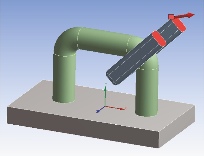
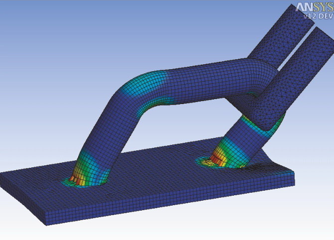
Подъемная скоба под действием растягивающего напряжения с последующим разрушением

Моделирование дроп-теста печатной платы
Возможности ANSYS Explicit Dynamics
ANSYS Explicit Dynamics по сути является актуальным препостом к решателю AUTODYN, а по этому обладает и его основными возможностями:
- Расчеты быстропротекающих высоко нелинейных процессов в постановках Лагранжа и Эйлера
- Моделирование процессов с участием жидкостей при помощи постановки Эйлера
- Бесшовная интеграция в Workbench – все преимущества и удобства работы с Engineering Data, SpaceClaim, Design Exploration, Meshing и т.д.
- Модели материалов и данные для металлов, керамики, стекла, бетона, грунтов, взрывчатых веществ, воды, воздуха и многих других твердых тел, жидкостей и газов.
Расчеты, выполняемые при помощи ANSYS Explicit Dynamics
ANSYS Explicit Dynamics позволяет решать все основные задачи явной динамики и быстропротекающих процессов.
- Ударопрочность (дроп-тест), например, электронных устройств и товаров народного потребления.
- Высокоскоростные и низкоскоростные удары в различных областях, от производства спортивного инвентаря до авиакосмической промышленности.
- Высоко нелинейное пластическое деформирование, возникающее в процессе эксплуатации изделия или в производственных процессах.
- Задачи разрушаемого контакта, возникающего при склеивании и точечной сварке.